Gambar L.2 Time Series Plot IHSG

(1)

L1

LAMPIRAN

Berikut ini adalah plot untuk masing-masing pembanding reksa dana

Gambar L.1

Time Series Plot

nilai Inflasi

(2)

L2

Gambar L.3

Time Series Plot

Suku Bunga

(3)

L3

Gambar L.5

Time Series Plot

Obligasi

Berikut ini adalah hasil korelasi antara NAB reksa dana dengan nilai inflasi, Index

Harga Saham Gabungan (IHSG), suku bunga, kurs mata uang dan Obligasi:

Correlations: Reksa Dana (, Inflasi (X1t), IHSG (X2t), Suku Bunga (, Kurs Mata Ua,

Reksa Da Inflasi IHSG (X2 Suku Bun Kurs Mat Inflasi 0.075

0.658

IHSG (X2 0.966 0.150 0.000 0.375

Suku Bun -0.839 0.019 -0.732 0.000 0.913 0.000

Kurs Mat 0.551 0.124 0.621 -0.105 0.000 0.464 0.000 0.535

Obligasi -0.508 0.090 -0.350 0.865 0.239 0.001 0.598 0.034 0.000 0.154

(4)

L4

Berikut ini adalah regresi individu variabel inflasi, IHSG, suku bunga,

kurs mata uang dan obligasi dengan NAB reksa dana:

Regression Analysis: Reksa Dana (yt) versus Inflasi (XIt)

The regression equation is

Reksa Dana (yt) = 1508 + 20.8 Inf1asi (X1t) Predictor Constant Inflasi Coef 1507.71 20.77

SE Coef 35.13 46.46 T 42.91 0.45 P 0.000 0.658

S = 140.0 R-Sq 0.6% R-Sq(adj) = 0.0% Analysis of Variance

Source Regression Residual Error Total

OF 1 35 36

Unusual Observations Obs Inflasi Reksa Da 4 1.85 1318.4 32 1. 91 1712.5

SS 3918 686107 690025 Fit 1546.1 1547.4 MS 3918 19603

SE Fit 63.7 66.3 F 0.20 P 0.658 Residual -227.7 165.1

X denotes an observation whose X value gives i t large influence.

St Resid -1. 83 X 1.34 X

Regression Analysis: Reksa Dana (yt) versus IHSG (X2t)

Reksa Dana (yt) = 1149 + 0.519 IHSG (X2t)

Predictor Coef SE Coef T P

Constant 1148.73 17.86 64.31 0.000 IHSG (X2 0.51894 0.02355 22.03 0.000

S = 36.41 R-Sq 93.3% R-Sq(adj) = 93.1%

Analysis of Variance

OF 1 35 36

Unusual Observations Obs IHSG (X2 Reksa Da

1 443 1271.09 2 36 409 1178 1285.21 1691.47 SS 643629 46396 690025 Fit 1378.61 1360.80 1760.11 MS 643629 1326 F 485.53 p 0.000

SE Fit Residual 8.76 -107.52 9.37 -75.59 12.45 -68.64

R denotes an observation with a large standardized residual

(5)

L5

Regression Analysis: Reksa Dana (yt) versus Suku Bunga (X3t)

Reksa Dana (yt) = 2006 - 53.0 Suku Bunga (X3t)

Constant 2005.70 54.70 36.67 0.000 Suku Bun -53.014 5.806 -9.13 0.000

S = 76.35 R-Sq 70.4% R-Sq(adj) = 69.6%

DF 1 35 36

Unusual Observations Obs Suku Bun Reksa Da 1 14.4 1271.1 37 9.5 1668.2

SS 485981 204044 690025 Fit 1244.9 1501.5 MS 485981 5830

SE Fit 32.6 12.7 F 83.36 P 0.000 Residual 26.1 166.7

R denotes an observation with a large standardized residual X denotes an observation whose X value gives i t large influence.

St Resid 0.38 X 2.21R

Regression Analysis: Reksa Dana (yt) versus Kurs Mata Uang

(X4t)

Reksa Dana (yt) = - 49 + 0.166 Kurs Mata Uang (X4t)

Predictor Coef Constant -48.9 Kurs Mat 0.16580

S = 117.2 R-Sq Analysis of Variance

DF 1 35 36

Unusual Observations

SE Coef 402.0 0.04245 30.4% SS 209456 480569 690025 T -0.12 3.91

R-Sq(adj) =

MS 209456 13731 P 0.904 0.000 28.4% F 15.25 P 0.000

Obs Kurs Mat Reksa Da Fit 1508.4 1527.8 1559.3 1731.8

SE Fit Residual 1 9393 1271.1

2 3 37 9510 9700 10740 1285.2 1300.2 1668.2

19.5 -237.3 19.4 -242.6 21.8 -259.1 57.6 -63.6

R denotes an observation with a large standardized residual X denotes an observation whose X value gives i t large influence.

(6)

Regression Analysis: Reksa Dana (Yt) versus Obligasi (X5t)

Reksa Dana (yt) = 1868 - 33.7 Obligasi (X5t)

Constant 1867.9 101. 9 18.33 0.000 Obligasi -33.689 9.666 -3.49 0.001 S = 121. 0 R-Sq 25.8% R-Sq(adj) = 23.6% Analysis of Variance

Source Regression Residual Error Total DF 1 35 36 SS 177779 512246 690025 MS 177779 14636 F 12.15 P 0.001

Unusual Observations Obs Obligasi Reksa Da

1 15.4 1271.1

37 14.3 1668.2

Fit 1350.8

1386.5

SE Fit 52.4

43.0

Residual -79.7

281.7 R denotes an observation with a large standardized residual X denotes an observation whose X value gives i t large influence.

L6

St Resid -0.73 X 2.49R

Berikut ini adalah hasil

Regression

serentak antara NAB reksa dana

dengan nilai inflasi, Index Harga Saham Gabungan (IHSG), suku

bung a,

kurs

mata uang, dan obligasi:

Regression Analysis: Reksa Dana (Yt) versus Inflasi (X1t), IHSG (X2t), ...

Reksa Dana (yt) = 1129 - _{6.65 Inflasi (Xlt)} ₊_{0.310 IHSG (X2t)} - _{27.7 Suku Bunga (X3t)} ₊_{0.0421 Kurs Mata Uang (X4t)}

+ 2.82 Obligasi (X5t)

Predictor Coef SE Coef T P VIF

Constant 1129.12 97.96 11. 53 0.000

Inflasi -6.653 7.565 -0.88 0.386 1.1

IHSG (X2 0.30951 0.04779 6.48 0.000 11. 4

Suku Bun -27.735 8.498 -3.26 0.003 26.1

Kurs Mat 0.04210 0.01345 3.13 0.004 2.9

Obligasi 2.818 6.207 0.45 0.653 12.6

S = 21. 88 R-Sq 97.8% R-Sq(adj) = 97.5% Analysis of Variance

Source DF SS MS F P

Regression 5 675183 135037 282.06 0.000

Residual Error 31 14842 479

(7)

Source OF Seq SS Inflasi 1 3918 IHSG (X2 1 643131 Suku Bun 1 23368 Kurs Mat 1 4668

Obligasi 1 99

Unusual Observations Obs Inflasi Reksa Da

37 0.55 1668.20

x

Fit 1679.12

SE Fit 15.95

Residual -10.92

x

denotes an observation whose X value gives it large influence.

Durbin-Watson statistic = 0.79

L7

St Resid -0.73

Output coefficients regresi individu dengan menggunakan

software

SPss:

Coefficients"

Unstandardized Standardized

Coefficients Coefficients

Model B Std. Error Beta t Sig.

1 (Constant) 1507.707 35.135 42.912 .000

Inflasi 20.771 46.460 .075 .447 .658

a. Dependent Variable: Reksa Dana

Coefficients"

Model B Std. Error Beta t Sig.

1 (Constant) 1148.734 17.862 64.310 .000

IHSG .519 .024 .966 22.035 .000

a. Dependent Variable: Reksa Dana

Coefficients"

Model B Std. Error Beta t Sig.

1 (Constant) 2005.697 54.703 36.665 .000

Suku Bunga -53.014 5.806 -.839 -9.130 .000

(8)

L8

Coefficientsa

-48.917 402.048 -.122 .904

.166 .042 .551 3.906 .000

(Constant) Kurs Mata Uang Model

1

B Std. Error Unstandardized

Coefficients

Beta Standardized

Coefficients

t Sig.

Dependent Variable: Reksa Dana a.

Coefficientsa

1867.900 101.902 18.330 .000

-33.689 9.666 -.508 -3.485 .001

(Constant) Obligasi Model

1

Coefficients

Beta Standardized

Coefficients

t Sig.

Output coefficients regresi serentak dengan menggunakan

software SPSS

:

Coefficientsa

1129.119 97.964 11.526 .000

-6.653 7.565 -.024 -.879 .386

.310 .048 .576 6.477 .000

-27.735 8.498 -.439 -3.264 .003

.042 .013 .140 3.130 .004

2.818 6.207 .042 .454 .653

(Constant) Inflasi IHSG Suku Bunga Kurs Mata Uang Obligasi Model

1

Coefficients

Beta Standardized

Coefficients

t Sig.

(9)

L9

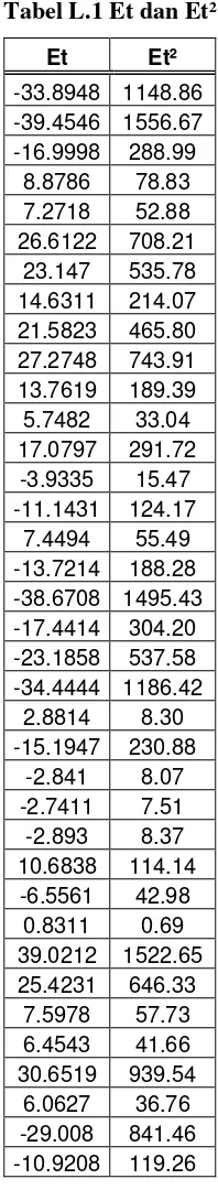
Berikut ini adalah data dari Et dan Et² persamaan regresi diatas:

Tabel L.1 Et dan Et²

Et Et²

-33.8948

1148.86

-39.4546

1556.67

-16.9998

288.99

8.8786 78.83

7.2718 52.88

26.6122 708.21

23.147 535.78

14.6311 214.07

21.5823 465.80

27.2748 743.91

13.7619 189.39

5.7482 33.04

17.0797 291.72

-3.9335 15.47

-11.1431

124.17

7.4494 55.49

-13.7214

188.28

-38.6708

1495.43

-17.4414

304.20

-23.1858

537.58

-34.4444

1186.42

2.8814 8.30

-15.1947

230.88

-2.841 8.07

-2.7411 7.51

-2.893 8.37

10.6838 114.14

-6.5561 42.98

0.8311 0.69

39.0212 1522.65

25.4231 646.33

7.5978 57.73

6.4543 41.66

30.6519 939.54

(10)

L10

(11)

L11

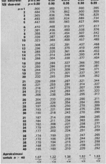
Tabel L.3 Kuartil-kuartil Statistik Uji Kolmogorov-Smirnov

Sumber

: L. H. Miller, Table of Percentage Points of Kolmogorov Statistics,”

J. Amer

.

Statist

.

(12)

L12

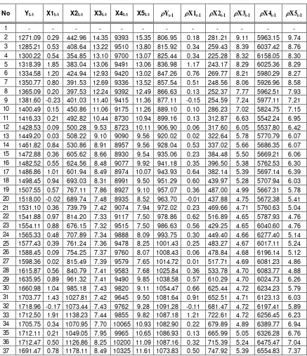
Tabel L.4 Hasil Perhitungan Transformasi Untuk Perbaikan Autokorelasi

No Yt-1 X1t-1 X2t-1 X3t-1 X4t-1 X5t-1 ρYt-1 ρX1t-1 ρX2t-1 ρX3t-1 ρX4t-1 ρX5t-1

1 - - -

(13)

L13

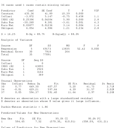
Berikut ini adalah hasil regresi setelah dilakukan perbaikan pada autokorelasi:

Regression Analysis: Reksa Dana ( versus Inflasi (X1, IHSG (X2), ...

Reksa Dana (Yt*) = 435 - 3.87 Inflasi (X1t*) + 0.254 IHSG (X2t*) - 30.3 Suku Bunga (X3t*) + 0.0388 Kurs Mata Uang (X4t*) + 6.05 Obligasi (X5t*)

36 cases used 1 cases contain missing values

Predictor Coef SE Coef T P VIF Constant 435.36 41.89 10.39 0.000

Inflasi -3.872 5.147 -0.75 0.458 1.1 IHSG (X2 0.25396 0.04304 5.90 0.000 2.8 Suku Bun -30.260 8.381 -3.61 0.001 4.3 Kurs Mat 0.03877 0.01236 3.14 0.004 1.4 Obligasi 6.054 4.986 1.21 0.234 2.8

S = 16.25 R-Sq = 89.7% R-Sq(adj) = 88.0%

Source DF SS MS F P Regression 5 69173 13835 52.42 0.000 Residual Error 30 7918 264

Total 35 77091

Source DF Seq SS Inflasi 1 0 IHSG (X2 1 63093 Suku Bun 1 2526 Kurs Mat 1 3164 Obligasi 1 389

Obs Inflasi Reksa Da Fit SE Fit Residual St Resid 30 0.77 649.30 607.57 5.20 41.73 2.71R 34 -0.01 629.21 597.64 4.39 31.57 2.02R 37 0.05 594.37 591.40 11.64 2.97 0.26X

R denotes an observation with a large standardized residual X denotes an observation whose X value gives it large influence.

(14)

L14

Output coefficients regresi individu dengan menggunakan

software SPSS

setelah

perbaikan autokorelasi:

Coefficientsa

564.397 8.512 66.306 .000

-.004 14.277 .000 .000 1.000

(Constant) Inflasi Model

1

B Std. Error Unstandardized Coefficients Beta Standardized Coefficients t Sig.

Coefficientsa

455.508 9.951 45.775 .000

.397 .034 .895 11.707 .000

(Constant) IHSG Model

1

Coefficientsa

718.054 27.993 25.651 .000

-47.869 8.537 -.693 -5.607 .000

(Constant) Suku Bunga Model

1

Coefficientsa

288.948 96.144 3.005 .005

.079 .028 .442 2.873 .007

(Constant) Kurs Mata Uang Model

1

(15)

L15

Coefficientsa

587.730 32.891 17.869 .000

-6.298 8.619 -.124 -.731 .470

(Constant) Obligasi Model

1

Coefficients

Beta Standardized

Coefficients

t Sig.

Output coefficients regresi dengan menggunakan

software SPSS

setelah perbaikan

autokorelasi:

Coefficientsa

435.364 41.887 10.394 .000

-3.872 5.147 -.047 -.752 .458

.254 .043 .573 5.901 .000

-30.260 8.381 -.438 -3.611 .001

.039 .012 .216 3.137 .004

6.054 4.986 .120 1.214 .234

(Constant) Inflasi IHSG Suku Bunga Kurs Mata Uang Obligasi Model

1

Coefficients

Beta Standardized

Coefficients

t Sig.

(16)

L16

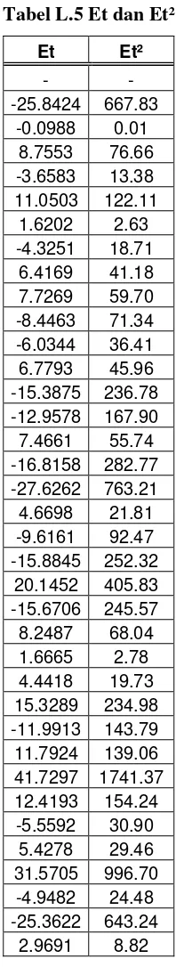
Berikut ini adalah data dari Et dan Et² persamaan regresi diatas:

Tabel L.5 Et dan Et²

Et Et²

- -

-25.8424

667.83

-0.0988 0.01

8.7553 76.66

-3.6583 13.38

11.0503 122.11

1.6202 2.63

-4.3251 18.71

6.4169 41.18

7.7269 59.70

-8.4463 71.34

-6.0344 36.41

6.7793 45.96

-15.3875

236.78

-12.9578

167.90

7.4661 55.74

-16.8158

282.77

-27.6262

763.21

4.6698 21.81

-9.6161 92.47

-15.8845

252.32

20.1452 405.83

-15.6706

245.57

8.2487 68.04

1.6665 2.78

4.4418 19.73

15.3289 234.98

-11.9913

143.79

11.7924 139.06

41.7297 1741.37

12.4193 154.24

-5.5592 30.90

5.4278 29.46

31.5705 996.70

-4.9482 24.48

-25.3622

643.24

(17)

L17

Berikut ini adalah hasil regresi untuk uji heteroskedastisitas sesudah dilakukan

perbaikan:

Regression Analysis: Et² versus Inflasi (X1t*), IHSG (X2t*), ...

Et² = 310 + 49 Inflasi (X1t*) + 1.04 IHSG (X2t*) + 3 Suku Bunga (X3t*) - 0.097 Kurs Mata Uang (X4t*) - 15 Obligasi (X5t*)

Inflasi 49.0 114.3 0.43 0.671 1.1 IHSG (X2 1.0389 0.9557 1.09 0.286 2.8 Suku Bun 2.6 186.1 0.01 0.989 4.3 Kurs Mat -0.0974 0.2745 -0.35 0.725 1.4 Obligasi -14.9 110.7 -0.13 0.894 2.8

S = 360.7 R-Sq = 10.3% R-Sq(adj) = 0.0%

Total 35 4353201

Obs Inflasi Et² Fit SE Fit Residual St Resid 30 0.77 1741.4 385.3 115.4 1356.1 3.97R 34 -0.01 996.7 297.5 97.4 699.2 2.01R 37 0.05 8.8 126.4 258.4 -117.6 -0.47X

(18)

L18

Tabel L.6 Hasil Perhitungan Transformasi Untuk Validasi ke-38 dan 39

t ρYt-1 ρX1t-1 ρX2t-1 ρX3t-1 ρX4t-1 ρX5t-1

38 1059.06 0.35 666.65 6.04 6818.29 9.07 39 983.12 0.44 652.56 6.35 6853.21 9.38

Berikut adalah regresi untuk validasi ke-38:

Regression Analysis: Reksa Dana ( versus Inflasi (X1t*, IHSG (X2t*), ...

Reksa Dana (Yt*) = 435 - 3.87 Inflasi (X1t*) + 0.254 IHSG (X2t*) - 30.3 Suku Bunga (X3t*) + 0.0388 Kurs Mata Uang (X4tt*) + 6.05 Obligasi (X5t*)

S = 16.25 R-Sq = 89.7% R-Sq(adj) = 88.0%

Total 35 77091

Predicted Values for New Observations

New Obs Fit SE Fit 95.0% CI 95.0% PI

1 594.65 7.52 (579.30, 610.01) (558.09, 631.21)

Values of Predictors for New Observations

(19)

L19

Berikut adalah regresi untuk validasi ke-39:

Regression Analysis: Reksa Dana ( versus Inflasi (X1t*, IHSG (X2t*), ...

Reksa Dana (Yt*) = 435 - 3.87 Inflasi (X1t*) + 0.254 IHSG (X2t*) - 30.3 Suku Bunga (X3t*) + 0.0388 Kurs Mata Uang (X4t*) + 6.05 Obligasi (X5t*)

S = 16.25 R-Sq = 89.7% R-Sq(adj) = 88.0%

Total 35 77091

Predicted Values for New Observations

New Obs Fit SE Fit 95.0% CI 95.0% PI

1 517.82 39.68 ( 436.79, 598.85) ( 430.26, 605.38) XX X denotes a row with X values away from the center

XX denotes a row with very extreme X values

Values of Predictors for New Observations

Gambar L.2 Time Series Plot IHSG

LAMPIRAN

Harga Saham Gabungan (IHSG), suku bunga, kurs mata uang dan Obligasi:

IHSG (X2 0.966 0.150 0.000 0.375

Berikut ini adalah regresi individu variabel inflasi, IHSG, suku bunga,

Regression Analysis: Reksa Dana (yt) versus IHSG (X2t)

Regression Analysis: Reksa Dana (yt) versus Kurs Mata Uang

Regression Analysis: Reksa Dana (Yt) versus Obligasi (X5t)

Berikut ini adalah hasil

Regression Analysis: Reksa Dana (Yt) versus Inflasi (X1t), IHSG (X2t), ...

Output coefficients regresi individu dengan menggunakan

Coefficients"

Model B Std. Error Beta t Sig.

Output coefficients regresi serentak dengan menggunakan

Coefficientsa

Berikut ini adalah data dari Et dan Et² persamaan regresi diatas:

Regression Analysis: Reksa Dana ( versus Inflasi (X1*, IHSG (X2*), ...

Output coefficients regresi individu dengan menggunakan

Coefficientsa

Coefficientsa

Output coefficients regresi dengan menggunakan

Coefficientsa

Berikut ini adalah data dari Et dan Et² persamaan regresi diatas:

Tabel L.6 Hasil Perhitungan Transformasi Untuk Validasi ke-38 dan 39

Berikut adalah regresi untuk validasi ke-39:

Regression Analysis: Reksa Dana ( versus Inflasi (X1, IHSG (X2), ...