Full Terms & Conditions of access and use can be found at
http://www.tandfonline.com/action/journalInformation?journalCode=ubes20
Download by: [Universitas Maritim Raja Ali Haji], [UNIVERSITAS MARITIM RAJA ALI HAJI
TANJUNGPINANG, KEPULAUAN RIAU] Date: 11 January 2016, At: 20:55
Journal of Business & Economic Statistics
ISSN: 0735-0015 (Print) 1537-2707 (Online) Journal homepage: http://www.tandfonline.com/loi/ubes20
HAC Corrections for Strongly Autocorrelated Time
Series
Ulrich K. Müller
To cite this article: Ulrich K. Müller (2014) HAC Corrections for Strongly Autocorrelated Time Series, Journal of Business & Economic Statistics, 32:3, 311-322, DOI:
10.1080/07350015.2014.931238
To link to this article: http://dx.doi.org/10.1080/07350015.2014.931238
Published online: 28 Jul 2014.
Submit your article to this journal
Article views: 567
View related articles
View Crossmark data
HAC Corrections for Strongly Autocorrelated
Time Series
Ulrich K. M ¨
ULLERDepartment of Economics, Princeton University, Princeton, NJ 08544 ([email protected])
Applied work routinely relies on heteroscedasticity and autocorrelation consistent (HAC) standard errors when conducting inference in a time series setting. As is well known, however, these corrections perform poorly in small samples under pronounced autocorrelations. In this article, I first provide a review of popular methods to clarify the reasons for this failure. I then derive inference that remains valid under a specific form of strong dependence. In particular, I assume that the long-run properties can be approximated by a stationary Gaussian AR(1) model, with coefficient arbitrarily close to one. In this setting, I derive tests that come close to maximizing a weighted average power criterion. Small sample simulations show these tests to perform well, also in a regression context.
KEYWORDS: AR(1); Local-to-unity; Long-run variance.
1. INTRODUCTION
A standard problem in time series econometrics is the deriva-tion of appropriate correcderiva-tions to standard errors when con-ducting inference with autocorrelated data. Classical references include Berk (1974), Newey and West (1987), and Andrews (1991), among many others. These articles show how one may estimate “heteroscedasticity and autocorrelation consis-tent” (HAC) standard errors, or “long-run variances” (LRV) in econometric jargon, in a large variety of circumstances.
Unfortunately, small sample simulations show that these cor-rections do not perform particularly well as soon as the underly-ing series displays pronounced autocorrelations. One potential reason is that these classical approaches ignore the sampling uncertainty of the LRV estimator (i.e.,t- andF-tests based on these corrections employ the usual critical values derived from the normal and chi-squared distributions, as if the true LRV was plugged in). While this is justified asymptotically under the assumptions of these articles, it might not yield accurate approximations in small samples.
A more recent literature, initiated by Kiefer, Vogelsang, and Bunzel (2000) and Kiefer and Vogelsang (2002a,2005), seeks to improve the performance of these procedures by explicitly taking the sampling variability of the LRV estimator into ac-count. (Also see Jansson 2004; M¨uller 2004, 2007; Phillips
2005; Phillips, Sun, and Jin2006,2007; Sun, Phillips, and Jin
2008; Gonalves and Vogelsang 2011; Atchade and Cattaneo
2012; Sun and Kaplan 2012.) This is accomplished by con-sidering the limiting behavior of LRV estimators under the as-sumption that the bandwidth is a fixed fraction of the sample size. Under such “fixed-b” asymptotics, the LRV estimator is no longer consistent, but instead converges to a random matrix. The resultingt- andF-statistics have limiting distributions that are nonstandard, with randomness stemming from both the param-eter estimator and the estimator of its variance. In these limiting distributions, the true LRV acts as a common scale factor that cancels, so that appropriate nonstandard critical values can be tabulated.
While this approach leads to relatively better size control in small sample simulations, it still remains the case that strong
underlying autocorrelations lead to severely oversized tests. This might be expected, as the derivation of the limiting distributions under fixed-b asymptotics assumes the underlying process to display no more than weak dependence.
This article has two goals. First, I provide a review of con-sistent and inconcon-sistent approaches to LRV estimation, with an emphasis on the spectral perspective. This clarifies why com-mon approaches to LRV estimation break down under strong autocorrelations.
Second, I derive valid inference methods for a scalar pa-rameter that remain valid even under a specific form of strong dependence. In particular, I assume that the long-run properties are well approximated by a stationary Gaussian AR(1) model. The AR(1) coefficient is allowed to take on values arbitrarily close to one, so that potentially, the process is very persistent. In this manner, the problem of “correcting” for serial correla-tion remains a first-order problem also in large samples. I then numerically determine tests about the mean of the process that (approximately) maximize weighted average power, using in-sights of Elliott, M¨uller, and Watson (2012).
By construction, these tests control size in the AR(1) model in large samples, and this turns out to be very nearly true also in small samples. In contrast, all standard HAC corrections have arbitrarily large size distortions for values of the autoregres-sive root sufficiently close to unity. In more complicated set-tings, such as inference about a linear regression coefficient, the AR(1) approach still comes fairly close to controlling size. Interestingly, this includes Granger and Newbold’s (1974) clas-sical spurious regression case, where two independent random walks are regressed on each other.
The remainder of the article is organized as follows. The next two sections provide a brief overview of consistent and inconsis-tent LRV estimation, centered around the problem of inference about a population mean. Section4 contains the derivation of the new test in the AR(1) model. Section5relates these results
© 2014American Statistical Association Journal of Business & Economic Statistics July 2014, Vol. 32, No. 3 DOI:10.1080/07350015.2014.931238
311
to more general regression and generalized method of moment (GMM) problems. Section6contains some small sample results, and Section7concludes.
2. CONSISTENT LRV ESTIMATORS
For a second-order stationary time series yt with
popula-tion meanE[yt]=μ,sample mean ˆμ=T−1Tt=1yt, and
ab-), a consistent estimator ofω2 allows the straightfor-ward construction of tests and confidence sets aboutμ.
It is useful to take a spectral perspective on the prob-lem of estimating ω2. The spectral density of yt is given by
the even function f : [−π, π]→[0,∞) defined via f(λ)= for notational convenience. The discrete Fourier transform is a one-to-one mapping from theT values{yt}T
t=1 into ˆμ, and the
The truly remarkable property of this transformation (see Propo-sition 4.5.2 in Brockwell and Davis1991) is that all pairwise cor-relations between theT random variablesT1/2
ˆ Thus, the discrete Fourier transform converts autocorrelation in
yt into heteroscedasticity of (Zsinl , Z
cos
l ), with the shape of the
heteroscedasticity governed by the spectral density.
This readily suggests how to estimate the LRVω2: collect the information about the frequency 2π l/T in thelth periodogram ordinate pl= 12((Zlcos)
2
+(Zsinl )2), so that pl becomes an
ap-proximately unbiased estimator of 2πf(2π l/T). Under the as-sumption thatf is flat over the frequencies [0,2π n/T] for some integer n, one would naturally estimate ˆωp,n2 =n−1n
l=1pl
(the subscriptpof ˆωp,n2 stands for “periodogram” ). Note that asymptotically, it is permissible to choosen=nT → ∞with nT/T →0, since any spectral density continuous at 0 becomes
effectively flat over [0,2π nT/T]. Thus, a law of large numbers
Popular consistent LRV estimators are often written as weighted averages of sample autocovariances, mimicking the
definition (1) Newey and West (1987) estimator, for instance, has this form withkequal to the Bartlett kernelk(x)=max(1− |x|,0). Up to some approximation ˆω2
k,ST can be written as a weighted average of periodogram ordinates
where the weights KT ,l approximately sum to one,
(T−1)/2
l=1 KT ,l →1. See Appendix for details. Since
(T /ST)KT ,lT =O(1) for lT =O(T /ST), these estimators are conceptionally close to ˆω2p,nT withnT ≈T /ST → ∞.
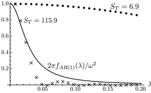
As an illustration, consider the problem of constructing a con-fidence interval for the population mean of the U.S. unemploy-ment rate. The data consist ofT =777 monthly observations and is plotted in the left panel ofFigure 1. The right panel shows the first 24 log-periodogram ordinates log(pj), along with the
corresponding part of the log-spectrum (scaled by 2π) of a fitted AR(1) process.
Now consider a Newey–West estimator with bandwidths cho-sen asST =0.75T1/3 ≈6.9 (a default value suggested in Stock
and Watson’s (2011) textbook for weakly autocorrelated data) andST =115.9 (the value derived in Andrews (1991) based on
the AR(1) coefficient 0.973). The normalized weightsKT ,l/KT ,1
of (5) for the first 24 periodogram ordinates, along with the AR(1) spectrum normalized by 2π/ω2, are plotted inFigure 2. Assuming the AR(1) model to be true, it is immediately apparent that both estimators are not usefully thought of as approximately consistent: the estimator withST =6.9 is severely downward
bi-ased, as it puts most of its weight on periodogram ordinates with expectation much belowω2.The estimator withS
T =115.9 is
less biased, but it has very substantial sampling variability, with 75% of the total weight on the first three periodogram ordinates. The example demonstrates that there is no way of solving the problem with a more judicious bandwidth choice: to keep the bias reasonable, the bandwidth has to be chosen very large. But such a large bandwidth makes ˆω2k,S
T effectively an average of very few periodogram ordinates, so that the LLN provides a very poor approximation, and sampling variability of ˆω2k,S
T cannot reasonably be ignored.
An alternative approach (Berk 1974; den Haan and Levin
1997) is to model yt as an autoregressive moving average
(ARMA) process with parameterθand spectrumfARMA(λ;θ),
say, and to estimateω2 from the implied spectrum ˆω2 ARMA =
2πfARMA(0; ˆθ).The discrete Fourier approximation (3) implies
Figure 1. U.S. unemployment. Notes: Series LNS14000000 of the Bureau of Labor Statistics from 1948:1 to 2012:9. The AR(1) log-spectral density has coefficient 0.973 and variance 0.182, the MLEs from a “low-frequency likelihood” (Equation (11) of Section 4 withq=48).
Whittle’s (1957,1962) log-likelihood approximation
T
2 log(2π)−
(T−1)/2
l=1
log(2πfARMA(2π l/T;θ))
−
(T−1)/2
l=1
pl
2πfARMA(2π l/T;θ)
to the Gaussian ARMA log-likelihood. The (quasi-) maximum likelihood estimator (MLE) ˆθthat defines ˆω2ARMAis thus deter-mined by information about all frequencies, as encoded by the whole periodogram. This is desirable if there are good reasons to assume a particular spectral shape foryt; otherwise, it leads
to potential misspecification, as ˆθmaximizes fit on average, but not necessarily for frequencies close to zero.
Also note that this approach only delivers a useful “con-sistent” estimator forω2 if the estimation uncertainty in ˆθ is
relatively small. The LRV of an AR(1) model, for instance, is given byω2
=σ2/(1
−ρ)2.This mapping is very sensitive
to estimation errors if ρ is close to one. As an illustration,
Figure 2. Newey–West weights on periodogram ordinates and nor-malized AR(1) spectral density. Notes: The dots and crosses correspond to the approximate weights on the first 24 periodogram ordinates of a Newey–West LRV estimator with bandwidth equal toST,
normal-ized by the weight on the first periodogram ordinate. Total weight
(T−1)/2
l=1 KT ,lis 0.99 and 0.85 forST =6.9 and 115.9, respectively.
The line is the spectral density of an AR(1) process with coefficient 0.973, scaled by 2π/ω2.
consider the AR(1) model for the unemployment series with
ρ=0.973. An estimation error of one standard error in ˆρ,
(1−ρ2)/T
≈0.008, leads to an estimation error in ˆωAR(1)2
by a factor of 0.6 and 2.0, respectively. So even if the AR(1) model was known to be correct over all frequencies, one would still expect ˆω2AR(1)to have poor properties forρclose to one.
A hybrid approach between kernel and parametric estima-tors is obtained by so-called prewhitening. The idea is to use a parsimonious parametric model to get a rough fit to the spectral density, and to then apply kernel estimator techniques to account for the misspecification of the parametric model near frequency zero. For instance, with AR(1) prewhitening, the overall LRV estimator is given by ˆω2
=ωˆ2
e/(1−ρˆ)2, where ˆρ is the
esti-mated AR(1) coefficient, and ˆω2
eis a kernel estimator applied to
the AR(1) residuals. Just as for the fully parametric estimator, this approach requires the estimation error in the prewhitening stage to be negligible.
3. INCONSISTENT LRV ESTIMATORS
The above discussion suggests that for inference with persis-tent time series, one cannot safely ignore estimation uncertainty in the LRV estimator. Under the assumption that the spectral density is approximately flat over some thin frequency band around zero, one might still rely on an estimator of the type
ˆ
ω2
p,n=n−
1n
l=1pl introduced in the last section. But in
con-trast to the discussion there, one would want to acknowledge that reasonable n are small, so that no LLN approximation holds. The randomness in thet-statistic√T( ˆμ−μ)/ωˆp,nthen
not only stems from the numerator, as usual, but also from the denominator ˆωp,n.
To make further progress, a distributional model for the peri-odogram ordinates is needed. Here, a central limit argument may be applied: under a linear process assumption foryt, say, the line
of reasoning in Theorems 10.3.1 and 10.3.2 of Brockwell and Davis (1991) implies that any finite set of the trigonometrically weighted averages (Zsinl , Zlcos) is asymptotically jointly normal. As a special case, the approximation (3) is thus strengthened to (Zsinl , Zlcos)′distributed approximately independent and normal with covariance matrix 2πf(2π l/T)I2,l=1, . . . , n. With an
assumption of flatness of the spectral density over the frequen-cies [0,2π n/T], that is, 2πf(2π l/T)≈ω2 for l
=1, . . . , n,
one therefore obtains ˆω2p,nto be approximately distributed chi-squared with 2n degrees of freedom, scaled byω2. Since the
common scale ω cancels from the numerator and denomina-tor, thet-statistic√T( ˆμ−μ)/ωˆp,nis then approximately
dis-tributed Student-twith 2ndegrees of freedom. The difference between the critical value derived from the normal distribution, and that derived from this Student-t distribution, accounts for the estimation uncertainty in ˆωp,n.
Very similar inconsistent LRV estimator have been suggested in the literature, although they are based on trigonometrically weighted averages slightly different from (Zsin
l , Z
cos
l ). In
partic-ular, the framework analyzed in M¨uller (2004,2007) and M¨uller and Watson (2008) led these authors to consider the averages
Yl =T−1/2
cosine weighted average of frequency just between 2π l/T and 2π(l+1)/T. This difference is quite minor, though: just like the discrete Fourier transform, (6) is a one-to-one transformation that maps{yt}Tt=1into theTvariables ˆμand{Yl}Tl=−11, andYl2is
an approximately unbiased estimator of the spectral density at frequency 2πf(π l/T). Under the assumption of flatness of the spectrum over the band [0, π q/T], and a CLT for{Yl}
q l=1, we
then obtain M¨uller’s (2004,2007) estimator
ˆ
which implies an approximate Student-tdistribution withq de-grees of freedom for thet-statistic√T( ˆμ−μ)/ωˆY,q. There is
an obvious trade-off between robustness and efficiency, as em-bodied by q: choosing q small makes minimal assumptions about the flatness of the spectrum, but leads to a very variable
ˆ
ω2
Y,q and correspondingly large critical value of thet-statistic √
T( ˆμ−μ)/ωˆY,q. Similar approaches, for potentially
differ-ent weighted averages, are pursued in Phillips (2005) and Sun (2013).
In the example of the unemployment series, one might, for instance, be willing to assume that the spectrum is flat below business cycle frequencies. Defining cycles of periodicity larger than 8 years as below business cycle, this leads to a choice of
qequal to the largest integer smaller than the span of the data in years divided by 4. In the example withT =777 monthly observations, (777/12)/4≈16.2,so thatq =16.Given the re-lationship betweenYland (Zlsin, Zlcos), this is roughly equivalent
to the assumption that the first eight periodogram ordinates in
Figure 1have the same mean. Clearly, if the AR(1) model with
ρ=0.973 was true, then this is a fairly poor approximation. At the same time, the data do not overwhelmingly reject the notion that {Yl}16l=1 is iid mean-zero normal: M¨uller and
Wat-son’s (2008) low-frequency stationarity test, for instance, fails to reject at the 5% level (although it does reject at the 10% level). The inconsistent LRV estimators that arise by settingST = bT for some fixedbin (4) as studied by Kiefer and Vogelsang (2005) are not easily cast in purely spectral terms, as Equation (5) no longer provides a good approximation whenST =bT in
general. Interestingly, though, the original (Kiefer, Vogelsang,
and Bunzel2000; Kiefer and Vogelsang2002b) suggestion of a Bartlett kernel estimator with bandwidth equal to the sample size can be written exactly as
ˆ
details). Except for an inconsequential scale factor, the estima-tor ˆω2KVB is thus conceptually close to a weighted average of periodogram ordinates (5), but with weights 1/(π l)2that do not spread out even in large samples. The limiting distribution un-der weak dependence is nondegenerate and equal to a weighted average of chi-square-distributed random variables, scaled by
ω2. Sixty percent of the total weight is onY2
KVB can also usefully be thought of as a
close cousin of (7) withqvery small.
As noted above, inference based on inconsistent LRV es-timators depends on a distributional model for ˆω2,
gener-ated by CLT arguments. In contrast, inference based on con-sistent LRV estimators only requires the LLN approxima-tion to hold. This distincapproxima-tion becomes important when con-sidering nonstationary time series with pronounced hetero-geneity in the second moments. To fix these ideas, suppose
yt =μ+(1+1[t > T /2])εt withεt ∼iid(0, σ2), that is, the
variance ofyt quadruples in the second half of the sample. It
is not hard to see that despite this nonstationarity, the estima-tor (4) consistently estimatesω2
=limT→∞var[T1/2μˆ]= 52σ 2,
so that standard inference is justified. At the same time, the nonstationarity invalidates the discrete Fourier approximation (3), so that {(Zsin
l , Z
cos
l )′} n
l=1 are no longer uncorrelated, even
in large samples, and√T( ˆμ−μ)/ωˆp,nis no longer distributed
and also the asymptotic approximations derived in Kiefer and Vogelsang (2005) for fixed-bestimators are no longer valid. In general, then, inconsistent LRV estimators require a strong de-gree of homogeneity to justify the distributional approximation of ˆω2, and are not uniformly more “robust” than consistent ones. One exception is the inference method suggested by Ibragi-mov and M¨uller (2010). In their approach, the parameter of in-terest is estimatedqtimes onqsubsets of the whole sample. The subsets must be chosen in a way that the parameter estimators are approximately independent and Gaussian. In a time series setting, a natural default for the subsets is a simple partition of the T observations into q nonoverlapping consecutive blocks of (approximately) equal length. Under weak dependence, the q resulting estimators of the mean ˆμl are asymptotically
independent Gaussian with meanμ. The variances of ˆμl are
approximately the same (and equal toqω2/T) when the time series is stationary, but are generally different from each other when the second moment of yt is heterogenous in time.
The usual t-statistic computed from the q observations ˆμl, l=1, . . . , q,
distribution as a t-statistic computed from independent and
zero-mean Gaussian variates of potentially heterogenous vari-ances. Now Ibragimov and M¨uller (2010) invoked a remarkable result of Bakirov and Sz´ekely (2005), who showed that ignoring potential variance heterogeneity in the small samplet-test about independent Gaussian observations, that is, to simply employ the usual Student-tcritical value withq−1 degrees of freedom, still leads to valid inference at the 5% two-sided level and below. Thus, as long asytis weakly dependent, simply comparing (9)
to a Student-tcritical value withq−1 degrees of freedom leads to approximately correct inference by construction, even under very pronounced forms of second moment nonstationarities in
yt. From a spectral perspective, the choice ofqin (9) roughly
corresponds to an assumption that the spectral density is flat over [0,1.5π q/T]. The factor of 1.5 relative to the assumption justifying ˆω2
Y,qin (7) reflects the relatively poorer frequency
ex-traction by the simple block averages ˆμl relative to the cosine
weighted averagesYl. See M¨uller and Watson (2013) for related
computations.
4. POWERFUL TESTS UNDER AR(1) PERSISTENCE
All approaches reviewed in the last two sections exploit flat-ness of the spectrum close to the origin: the driving assumption is that there are at least some trigonometrically weighted aver-ages that have approximately the same variance as the simple average√Tμˆ. But asFigure 2demonstrates, there might be only very few, or even no such averages for sufficiently persistentyt.
An alternative approach is to take a stand on possible shapes of the spectrum close to the origin, and to exploit that restric-tion to obtain better estimators. The idea is analogous to using a local polynomial estimator, rather than a simple kernel es-timator, in a nonparametric setting. Robinson (2005) derived such consistent LRV estimators under the assumption that the underlying persistence is of the “fractional” type. This section derives valid inference when instead the long-run persistence is generated by an autoregressive root close to unity. In contrast to the fractional case, this precludes consistent estimation of the spectral shape, even if this parametric restriction is imposed on a wide frequency band.
4.1. Local-To-Unity Asymptotics
For very persistent series, the asymptotic independence be-tween{(Zsinl , Zlcos)′}nl=1, or{Yl}
q
l=1, no longer holds. So we
be-gin by developing a suitable distributional theory for{Yl} q l=0for
fixedq, whereY0=
√ Tμˆ.
Suppose initially thatyt is exactly distributed as a
station-ary Gaussian AR(1) with meanμ, coefficient ρ,|ρ|<1, and varianceσ2: withy
=(y1, . . . , yT)′ande=(1, . . . ,1)′, y ∼N(μe, σ2
(ρ)),
where(ρ) has elements(ρ)i,j =ρ|i−j|/(1−ρ2). DefineH
as theT ×(q+1) matrix with first column equal to T−1/2e, and (l+1)th column with elements T−1/2√2 cos(π l(t−
1/2)/T), t=1, . . . , T, and ι1 as the first column of Iq+1.
Then Y =(Y0, . . . , Yq)′=H′y ∼N(T1/2μι1, σ2(ρ)) with
(ρ)=H′(ρ)H.
The results reviewed above imply that for any fixed q and
|ρ|<1, asT → ∞,σ2(ρ) becomes proportional toI
q+1(with
proportionality factor equal toω2=σ2/(1−ρ)2). But for any fixedT, there exists aρsufficiently close to one for which(ρ) is far from being proportional toIq+1. This suggests that
asymp-totics along sequencesρ=ρT →1 yield approximations that
are relevant for small samples with sufficiently largeρ. The appropriate rate of convergence of ρT turns out to be ρT =1−c/T for some fixed number c >0, leading to
so-called “local-to-unity” asymptotics. Under these asymptotics, a calculation shows that T−2(ρ
T)→0(c), where the (l+
1),(j +1) element of0(c) is given by
1 2c
1
0
1
0
φl(s)φj(r)e−c|r−s|dsdr (10)
withφl(s)= √
2 cos(π ls) forl≥1 andφ0(s)=1 . This
expres-sion is simply the continuous time analogue of the quadratic formH′(ρ)H: the weighting functionsφl corresponds to the
limit of the columns ofH,T(1−ρT2)→2cande−c|r−s| corre-sponds to the limit ofρ|i−j|.
Now the assumption that yt follows exactly a stationary
Gaussian AR(1) is obviously uncomfortably strong. So suppose instead that yt is stationary and satisfies yt=ρTyt−1+(1−
ρT)μ+ut, whereutis some weakly dependent mean-zero
dis-turbance with LRV σ2. Under suitable conditions, Chan and
Wei (1987) and Phillips (1987) showed thatT−1/2(y
[·T]−μ)
then converges in distribution to an Ornstein–Uhlenbeck process
σ Jc(·), with covariance kernel E[Jc(r)Jc(s)]=e−c|r−s|/(2c).
Noting that this is exactly the kernel in (10), the approximation
T−1Y ∼N(T−1/2μι1, σ20(c)) (11)
is seen to hold more generally in large samples. The di-mension of Y, that is, the choice of q, reflects over which frequency band the convergence to the Ornstein–Uhlenbeck process is deemed an accurate approximation (see M¨uller
2011 for a formal discussion of asymptotic optimality un-der such a weak convergence assumption). Note that for largec,e−c|r−s| in (10) becomes very small for nonzero |r− s|, so that 1
0
1
0 φl(s)φj(r)e−
c|r−s|dsdr∝1
0 φl(s)φj(s)ds=
1[i=j], recovering the proportionality of 0(c) to Iq+1 that
arises under a spectral density that is flat in the 1/T neigh-borhood of the origin. For a given q, inference that remains valid under (11) for allc >0 is thus strictly more robust than
t-statistic-based inference with ˆω2
Y,qin (7).
4.2. Weighted Average Power Maximizing Scale Invariant Tests
Without loss of generality, consider the problem of testing
H0:μ=0 (otherwise, simply subtract the hypothesized mean
fromyt) againstH1:μ=0,based on the observationY with
distribution (11). The derivation of powerful tests is complicated by the fact that the alternative is composite (μis not specified underH1), and the presence of the two nuisance parametersσ2
andc.
A useful device for dealing with the composite nature of the alternative hypothesis is to seek tests that maximize weighted av-erage power. For computational convenience, consider a weight-ing function forμthat is mean-zero Gaussian with varianceη2.
As argued by King (1987), it makes sense to choose η2 in a
way that good tests have approximately 50% weighted aver-age power. Now forcandT large, var[T−1Y
0]≈T−2σ2/(1−
ρT)2≈σ2/c2. Furthermore, if σ andcwere known, the best
5% level test would simply reject if |T−1Y
0|>1.96·σ/c.
This motivates a choice of η2=10T σ2/c2, since this would induce this (infeasible) test to have power of approximately 2P(N(0,11)>1.96)≈56%. Furthermore, by standard argu-ments, maximizing this weighted average power criterion for givenσ andcis equivalent to maximizing power against the alternative
T−1Y ∼N(0, σ21(c)) (12)
with1(c)=0(c)+(10/c2)ι1ι′1.
The testing problem has thus been transformed into H′
0:
T−1Y
∼N(0, σ2
0(c)) against H1′ :T− 1Y
∼N(0, σ2 1(c)),
which is still complicated by the presence of the two nuisance parametersσ2 andc. Forσ2, note that in most applications, it
makes sense to impose that if the null hypothesis is rejected for some observationY, then it should also be rejected for the ob-servationaY, for anya >0. For instance, in the unemployment example, this ensures that measuring the unemployment rate as a ratio (values between 0 and 1) or in percent (values between 0 and a 100) leads to the same results. Standard testing theory (see chap. 6 in Lehmann and Romano2005) implies that any test that satisfies this scale invariance can be written as a function ofYs=Y /√Y′Y. One might thus think ofYs as the effective
observation, whose density underH′
i,i=0,1 is equal to (see
Kariya1980; King1980)
fi,c(ys)=κq|i(c)|−1/2(ys′i(c)−1ys)−(q+1)/2 (13)
for some constantκq.
A restriction to scale invariant tests has thus further trans-formed the testing problem into H′′
0 :“Ys has density f0,c”
againstH′′
1 : “Yshas densityf1,c.” This is a nonstandard
prob-lem involving the key nuisance parameterc >0, which governs the degree of persistence of the underlying time series. Elliott, M¨uller, and Watson (2012) studied nonstandard problems of this kind, and showed that a test that approximately maximizes weighted average power relative to the weighting function F
rejects for large values of f1,c(Ys)dF(c)/
f0,c(Ys)d˜(c),
where ˜ is a numerically determined approximately least favorable distribution. I implement this approach with F dis-crete and uniform on the 15 pointscj =e(j−1)/2,j =1, . . . ,15,
so that weighted average power is approximately maximized against a uniform distribution on log(c) on the interval [0,7]. The endpoints of this interval are chosen such that the whole span of very nearly unit root behavior (c=1) to very nearly stationary behavior (c=e7
≈1097) is covered. The substantial mass on relatively large values ofcinduces good performance also under negligible degrees of autocorrelation.
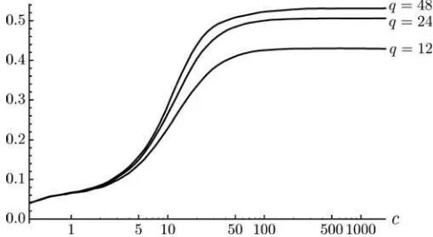
Figure 3plots the power of these tests forq∈ {12,24,48}
against the alternatives (12) as a function of log(c). As can be seen from Figure 3, none of these tests have power when
c→0. To understand why, go back to the underlying station-ary AR(1) model for yt. For small c (say,c <1), yt−y1 is
essentially indistinguishable from a random walk process. De-creasing cfurther thus leaves the distribution of {yt−y1}Tt=1
largely unaffected, while it still increases the variance of y1,
var[y1]=σ2/(1−ρT2)≈σ
2T /(2c). But for a random walk, the
Figure 3. Asymptotic weighted average power of tests under AR(1) persistence. Notes: Asymptotic weighted average power of 5% level hypothesis tests about the mean of an AR(1) model with unit innova-tion variance and coefficientρ=ρT =1−c/Twith anN(0,10T /c2)
weighting function on the difference between population and hypothe-sized mean, based onqlow-frequency cosine weighted averages of the original data.
initial conditiony1−μand the meanμare not separately
iden-tified, as they both amount to translation shifts. With the mean-zero Gaussian weighting onμ, and under scale invariance, the alternativeH1′′:“Ys has densityf
1,c” for some smallc=c1is
thus almost indistinguishable from the nullH0′′: “Yshas density
f0,c0” for somec0< c1, so that power under such alternatives cannot be much larger than the nominal level. As a consequence, if the tests are applied to an exact unit root process (c=0, which is technically ruled out in the derivations here) with arbitrary fixed initial condition, they only reject with 5% probability. This limiting behavior might be considered desirable, as the population mean of a unit root process does not exist, so a valid test should not systematically rule out any hypothesized value.
The differences in power for different values ofqinFigure 3
reflect the value of the additional information contained inYl,l
large, for inference aboutμ. This information has two compo-nents: on the one hand, additional observationsYl help to pin
down the common scale, analogous to the increase in power of tests based on ˆωY,q2 in (7) as a function ofq. On the other hand, additional observationsYl contain information about the shape
parameterc. For instance, as noted above,c→ ∞corresponds to flatness of the spectral density in the relevant 1/T neigh-borhood of the origin. The tests based on ˆω2Y,q dogmatically impose this flatness and have power of{52.4%, 54.0%, 54.7%} forq ∈ {12,24,48}against the alternative (12) withc→ ∞. Forq=12 , this power is 9.4% larger than the power of the test inFigure 3forclarge, reflecting that 12 observations are not sufficient to learn about the flatness of the spectrum. For
q=24 andq =48, however, the difference is only 3.3% and 1.6%, respectively.
Even withq→ ∞, the shape of the spectral density cannot be consistently estimated under local-to-unity asymptotics. In unreported results, I derive weighted average power maximizing tests based on all observations of a Gaussian AR(1), and find that asymptotic overall weighted average power in thisq= ∞
case is only 1.9% larger than what is obtained withq =48. As a practical matter, it thus makes little sense to consider tests with
qlarger than 48.
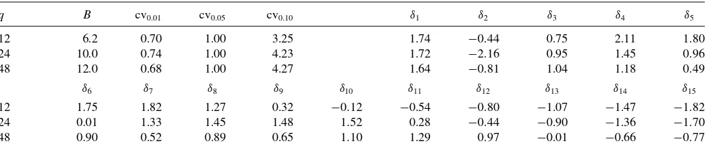
Table 1. Constants for computation ofSq
4.3. Suggested Implementation and Empirical Illustration
The suggested test statistic is a slightly modified version of
f1,c(Ys)dF(c)/
f0,c(Ys)d˜(c). A first modification
approx-imates0(c) by diagonal matrices with elements 1/(c2+π2j2);
these diagonal values correspond to the suitably scaled limit of the spectral density of an AR(1) process with ρ=ρT =
1−c/T at frequencyπj/T. This avoids the slightly cumber-some determination of the elements of0(c) as a double integral
in (10). The second modification bounds the value of|Y0|relative
to (Y1, . . . , Yq)′. The bound is large enough to leave weighted
average power almost completely unaffected, but it eliminates the need to include very small values of cin the support of
˜
, and helps to maintain the power of the test against distant alternatives whencis large. (Without this modification, it turns out that power functions are not monotone forclarge.) Taken together, these modifications lead to a loss in overall weighted average power relative to the 5% level test reported inFigure 3
of approximately one percentage point for all considered values ofq.
In detail, the suggested test about the population meanH0:
μ=μ0of an observed scalar time series{yt}Tt=1is computed as
inTable 1. (For reasons described above.)
3. Definedi,l0 =(c2i +(π l)2)/ci2, whereci=e(i−1)/2, anddi,l1 = di,l0 for l≥1, and di,10=1/11, i=1, . . . ,15. (These are the elements of the diagonal approximations to0(c)−1and
1(c)−1, scaled by 1/c2for convenience.)
sponds to the ratio of
f1,c(Ys)dF(c)/
Table 1. (The 5% level critical values are all equal to one, as the appropriate cut-off value for the (approximate) ratio
f1,c(Ys)dF(c)/
f0,c(Ys)d˜(c) is subsumed inδi.)
The values ofB,δi, and cvαare numerically determined such
that the testSqis of nominal level under (11), for arbitraryc >0,
and that it come close to maximizing weighted average power relative to the weighting functionFand (12) at the 5% level.
A confidence interval forμcan be constructed by inverting this test, that is, by determining the set of values ofμ0for which
the test does not reject. This is most easily done by a simple grid search over plausible values ofμ0(note that different values of
μ0leaveYl,l≥1 unaffected). Numerical calculations suggest
that 95% confidence intervals are never empty, asSq does not
seem to take on values larger than the critical value whenever
Y0=0, that is, whenμ0=μˆ. They can be equal to the real
line, though, asSq might not reject for any value ofμ0. When
ρis very close to one (cis very small), this happens necessarily for almost 95% of the draws, as such series contain essentially no information about the population mean. Under asymptotics that correspond to weak dependence (c→ ∞), unbounded 95% confidence intervals still arise for 8.6% of the draws by inverting
S12, but essentially never (<0.05%) when invertingS24orS48.
Table 2reports 95% confidence intervals for the population mean of U.S. unemployment using this test. As a comparison, the table also includes 95% confidence intervals based on three “consistent” estimators (i.e., standard normal critical values are employed) and five “inconsistent” estimators. Specifically, the first group includes Andrews’ (1991) estimator ˆω2A91 with a quadratic spectral kernel k and bandwidth selection using an AR(1) model; Andrews and Monahan’s (1992) ˆω2AMsuggestion of the same estimator, but after prewhitening with an AR(1) model; and the fully parametric estimator ˆω2
AR(12)based on an
Table 2. 95% confidence intervals for unemployment population mean
S12 S24 S48 ωˆA912 ωˆ
NOTES: Unemployment data same as inFigure 1. All confidence intervals are symmetric around the sample mean ˆμ=5.80 with endpoints ˆμ±m.e., where the margin of error m.e. is reported in the table.
AR(12) model. The second group includes Kiefer, Vogelsang, and Bunzel’s (2000) Bartlett kernel estimator with lag-length equal to sample size ˆω2
KVB; M¨uller’s (2007) estimators ˆωY,212and
ˆ
ω2Y,24; Sun, Phillips, and Jin’s (2008) quadratic spectral estimator ˆ
ω2SPJwith a bandwidth that trades off asymptotic Type I and Type II errors in rejection probabilities, with the shape of the spectral density approximated by an AR(1) model and with their weight parameterw equal to 30; and Ibragimov and M¨uller’s (2010) inference with 8 and 16 groups, IM8and IM16. The confidence
interval based on S12 is equal to the whole real line; the 12
lowest cosine transforms (6) of the unemployment rate do not seem to exhibit sufficient evidence of mean reversion for the test to reject any value of the population mean. The full sample AR(1) coefficient estimate is equal to 0.991; this very large value seems to generate the long intervals based on ˆω2AMand ˆω2SPJ.
5. GENERALIZATION TO REGRESSION AND GMM PROBLEMS
The discussion of HAC corrections has so far focused on the case of inference about the meanμof an observable time series
{yt}Tt=1. But the approaches can be generalized to inference about
scalar parameters of interest in regression and GMM contexts. Consider first inference about a regression parameter. Denote byβ thek×1 regression coefficient, and suppose we are in-terested in its first elementβ1=ι′1β, where in this section,ι1
denotes the first column ofIk. The observable regressandRtand k×1 regressorsXtare assumed to satisfy
Rt =X′tβ+et, E[et|Xt−1, Xt−2, . . .]=0, t=1, . . . , T .
able regular conditions, ˆX p
X Xtet. The problem of estimating the variance
of ˆβ1is thus cast in the form of estimating the LRV of the scalar
series ˜yt.
The series ˜ytis not observed, however. So consider instead the
observable series ˆyt =ι′1ˆ− 1
X Xteˆt, with ˆet =Rt−Xt′βˆthe OLS
residual, and suppose the HAC corrections discussed in Sections
2 and 3 are computed foryt =yˆt. The difference between ˜yt
is asymptotically negligible. Furthermore, since ˆβ→p β, the last term cannot substantially affect many periodogram ordinates at the same time, so that forconsistentLRV estimators the under-lying LLN still goes through. Forinconsistentestimators, one obtains the same result as discussed in Section 3 if averages ofXtXt′are approximately the same in all parts of the sample,
(rT −sT)−1rT
t=sT+1XtX′t p
→X, for all 0≤s < r ≤1.
Un-der this homogeneity assumption, ˆ−X1XtX′t averages in large
samples toIk when computing Fourier transforms (2), or
co-sine transforms (6), for any fixed l. Thus, ˆyt behaves just
like the demeaned series ˜yt−T−1 T
s=1y˜s≈y˜t−( ˆβ1−β1).
Consequently, ˆω2p,n, ˆω2Y,q, or ˆω2KVBcomputed fromyt =yˆt are
asymptotically identical to the infeasible estimators computed fromyt =y˜t, as the underlying weights are all orthogonal to a
constant. One may thus rely on the same asymptotically justi-fied critical values; for instance, under weak dependence, the
t-statistic√T( ˆβ1−β1)/ωˆY,qis asymptotically Student-twithq
degrees of freedom.
The appropriate generalization of the Ibragimov and M¨uller (2010) approach to a regression context requiresqestimations of the regression on theqblocks of data, followed by the com-putation of a simplet-statistic from theqestimators ofβ1.
For the testsSq derived in Section4, suppose the hypothesis
to be tested isH0:β1 =β1,0. One would expect that under the
null hypothesis, the product of the OLS residuals of a regres-sion ofRt−ι′1Xtβ1,0andι′1XtonP Xt, respectively, where the k×(k−1) matrixPcollects the lastk−1 columns ofIk, forms
a mean-zero series, at least approximately. Some linear regres-sion algebra shows that this product, scaled by 1/ι′
1ˆ−
Thus, the suggestion is to compute (15), followed by the imple-mentation described in Section4.3. IfXt =1, this reduces to
what is suggested there for inference about a population mean. The construction of the tests Sq assumes yt to have
low-frequency dynamics that resemble those of a Gaussian AR(1) with coefficient possibly close to one, and that alternatives cor-respond to mean shifts of yt. This might or might not be a
useful approximation under (15), depending on the long-run properties ofXt andet. For instance, if Xt and et are scalar
independent stationary AR(1) processes with the same coeffi-cient close to unity, thenyt in (15) follows a stationary AR(1)
with a slightly smaller coefficient, but it is not Gaussian, and incorrect values ofβ1,0 do not amount to translation shifts of
yt. Neither the validity nor the optimality of the testsSq thus
goes through as such. One could presumably derive weighted average power maximizing tests that are valid by construction for any particular assumption of this sort. But in practice, it is difficult to specify strong parametric restrictions for the joint long-run behaviorXtandet. And for any given realizationXt, ytin (15) may still follow essentially any mean-zero process via
a sufficiently peculiar conditional distribution of{et}Tt=1 given
{Xt}Tt=1. Finally, under the weak dependence and homogeneity
assumptions that justify inconsistent estimators in a linear re-gression context,Ylforl≥1 computed from ˆyt =ι′1ˆ−
1
X Xteˆt,
andYlcomputed fromytin (15), are asymptotically equivalent,
and they converge to mean-zero-independent Gaussian variates of the same variance as√T( ˆβ1−β1). Since iid GaussianYl
cor-responds to the special case ofc→ ∞in the analysis of Section
4, the testsSq are thus also valid under such conditions. So as
practical matter, the testsSqunder definition (15) might still be
useful to improve the quality of small sample inference, even if the underlying assumptions are unlikely to be met exactly for finitecin a regression context.
Now consider a potentially overidentified GMM problem. Letθ be thek×1 parameter, and suppose the hypothesis of interest concerns the scalar parameterθ1=ι′1θ,H0 :θ1 =θ1,0.
Let ˆθ be the k×1 GMM estimator, based on the r×1 moment condition gt(θ) with r×k derivative matrix ˆG= T−1T
t=1∂gt(θ)/∂θ′|θ=θˆ andr×r weight matrix W. In this
notation, the appropriate definition for ˆytis
ˆ
yt = −ι′1( ˆG′WGˆ)− 1ˆ
G′W gt( ˆθ).
For the analogue ofyt, define ˆθ0as the GMM estimator under
the constraintθ1=θ1,0, and ˆG0 =T−1
T
t=1∂gt(θ)/∂θ′|θ=θˆ0. Then set
yt = −ι′1( ˆG 0′WGˆ0
)−1Gˆ0′W gt( ˆθ0).
These definitions reduce to what is described above for the special case of a linear regression.
6. SMALL SAMPLE COMPARISON
This section contains some evidence on the small sample size and power performance of the different approaches to HAC corrections.
In all simulations, the sample size is T =200. The first two simulations concern the mean of a scalar time series. In the “AR(1)” design, the data are a stationary Gaussian AR(1) with coefficient ρ and unit innovation variance. In the “AR(1)+Noise” design, the data are the sum of such an AR(1) process and independent Gaussian white noise of variance 4.
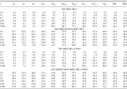
Table 3 reports small sample size and size-adjusted power of the same 12 two-sided tests of 5% nominal level that were reported inTable 2 of Section4.3in the unemployment illus-tration. Due to the much smaller sample size in the simula-tion, the parametric estimator ˆω2
AR is based on 4 lags,
how-ever. The size-adjustment is performed on the ratio of test statistic and critical value; this ensures that data-dependent critical values are appropriately subsumed in the effective test.
The AR(1) design is exactly the data-generating process for which the testSqwas derived, and correspondingly, size control
is almost exact. All other approaches lead to severely oversized tests as ρ becomes large. (All LRV estimators ˆω2 considered
here are translation invariant, so that for fixedT, they have a well-defined limiting distribution asρ→1. At the same time, for any
M,P(|μˆ−μ|> M)→1 asρ→1. Thus, all LRV-based tests have arbitrarily poor size control forρsufficiently close to one, and the same also holds for the IMq tests.) By construction,
Table 3. Small sample performance for inference about population mean
ρ S12 S24 S48 ωˆ2A91 ωˆ2AM ωˆ2AR(4) ωˆ2KVB ωˆ2Y,12 ωˆY2,24 ωˆSPJ2 IM8 IM16
Size under AR(1)
0.0 4.7 4.9 5.0 5.5 5.5 6.7 5.0 5.2 5.2 5.1 5.1 5.1 0.7 4.9 4.9 5.0 10.0 7.0 8.1 6.1 6.3 8.8 5.5 6.0 8.1 0.9 5.0 4.8 5.3 17.2 10.7 12.0 8.9 13.8 24.7 6.6 10.5 19.1 0.95 5.0 5.0 5.1 25.5 15.3 16.8 13.0 25.8 41.3 8.8 18.6 32.8 0.98 4.9 4.7 5.0 44.2 26.5 27.7 23.0 48.3 62.0 13.0 37.3 54.3 0.999 4.8 4.6 4.5 87.7 68.1 68.7 71.2 88.1 92.0 44.5 84.3 89.7
Size-adjusted power under AR(1)
0.0 35.7 42.8 47.1 50.0 49.9 47.6 37.3 44.3 47.4 48.8 40.1 45.8 0.7 34.8 41.7 44.8 46.4 47.0 45.1 36.2 45.1 47.8 39.9 41.5 46.4 0.9 28.8 34.5 35.6 42.7 41.4 41.9 34.7 46.4 48.5 31.6 42.7 46.7 0.95 21.0 23.2 25.3 40.3 38.5 38.6 33.9 46.9 48.5 27.9 43.6 47.0 0.98 11.3 12.5 12.2 40.0 38.1 37.6 35.1 51.4 52.9 26.9 47.2 51.4 0.999 5.6 5.6 5.6 92.6 74.3 73.9 80.0 98.5 99.0 53.6 97.4 98.5
Size under AR(1)+Noise
0.0 4.6 4.7 4.8 5.3 5.3 6.4 4.8 5.1 4.7 4.8 4.9 5.0 0.7 4.9 5.2 5.9 12.6 13.1 8.1 5.9 5.8 7.4 6.4 5.8 7.1 0.9 5.2 5.7 9.5 27.7 37.5 14.5 8.8 12.8 23.1 10.6 10.0 17.8 0.95 5.3 6.7 12.6 38.0 52.4 21.1 12.8 25.5 40.1 15.9 18.3 31.8 0.98 5.4 7.1 15.1 52.5 67.9 33.6 23.1 47.9 61.5 26.3 37.3 53.8 0.999 5.4 7.4 17.7 86.2 91.9 73.6 71.1 88.1 91.9 68.0 84.2 89.6
Size-adjusted power under AR(1)+Noise
0.0 35.9 43.9 48.6 51.3 51.0 48.9 37.5 44.8 49.5 50.2 40.9 46.5 0.7 34.4 41.9 46.2 48.9 49.6 46.6 35.8 45.5 48.3 46.0 41.4 46.8 0.9 28.9 35.8 39.0 46.1 48.6 43.0 34.5 46.8 48.9 42.6 42.3 47.6 0.95 21.3 23.5 26.7 43.2 47.2 39.9 34.0 47.6 49.4 39.2 43.6 48.3 0.98 11.8 12.0 12.6 43.0 48.8 39.5 35.5 51.5 53.5 37.7 47.9 51.3 0.999 5.54 5.56 5.53 85.6 91.0 76.8 80.7 98.7 99.1 72.2 97.3 98.6
NOTES: Entries are rejection probability in percent of nominal 5% level tests. Under the alternative, the population mean differs from the hypothesized mean by 2T−1/2(1−ρ)−1and
2T−1/2(4+(1−ρ)−2)1/2, respectively. Based on 20,000 replications.
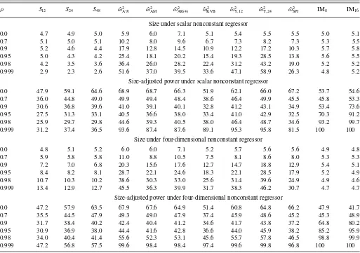
Table 4. Small sample performance for inference about regression coefficient
ρ S12 S24 S48 ωˆ2A91 ωˆ 2
AM ωˆ
2
AR(4) ωˆ
2
KVB ωˆ
2
Y,12 ωˆ 2
Y,24 ωˆ 2
SPJ IM8 IM16
Size under scalar nonconstant regressor
0.0 4.7 4.9 5.0 5.9 6.0 7.1 5.1 5.4 5.5 5.5 5.0 5.1 0.7 5.1 5.0 5.1 10.2 8.0 9.6 6.7 7.3 8.2 7.3 5.3 5.5 0.9 5.2 4.6 4.4 17.9 12.8 14.5 10.9 12.2 17.2 10.3 5.7 5.8 0.95 5.0 4.3 4.2 25.4 18.1 20.2 15.4 19.3 28.5 13.8 5.6 5.5 0.98 4.2 3.5 3.6 36.4 26.0 28.2 22.4 31.2 43.2 19.0 5.2 5.2 0.999 2.9 2.3 2.6 51.6 37.0 39.5 33.6 47.1 58.9 26.3 4.8 5.2
Size-adjusted power under scalar nonconstant regressor
0.0 47.9 59.1 64.6 68.9 68.7 66.3 51.9 62.1 66.0 67.2 53.7 54.6 0.7 36.0 44.8 49.0 49.9 49.4 48.4 38.6 46.4 49.9 45.5 45.8 53.3 0.9 30.6 36.8 39.6 41.0 39.1 40.1 32.8 41.2 43.1 34.9 53.4 73.6 0.95 27.5 31.3 33.1 40.5 36.6 38.0 33.4 41.0 42.9 32.5 70.3 91.2 0.98 25.9 29.7 29.8 44.6 39.3 40.5 38.0 46.4 48.7 34.6 93.2 99.7 0.999 31.2 37.4 36.5 93.6 87.4 87.6 89.1 95.3 95.8 81.5 100 100
Size under four-dimensional nonconstant regressor
0.0 4.8 5.1 5.2 6.0 6.0 7.1 5.2 5.7 5.6 5.6 4.9 4.8 0.7 5.9 5.8 5.8 11.0 8.8 10.5 7.5 8.1 8.6 8.0 5.3 5.3 0.9 7.2 7.0 6.8 20.3 15.6 17.6 12.7 14.7 18.8 12.9 5.4 5.1 0.95 8.4 8.2 8.1 28.7 22.1 24.6 18.3 22.1 28.5 17.9 5.2 4.9 0.98 10.7 10.3 10.2 38.6 30.3 33.0 25.6 31.4 39.6 24.9 4.9 4.6 0.999 13.4 12.9 12.7 45.5 36.3 39.9 31.7 38.3 46.2 30.7 4.7 4.7
Size-adjusted power under four-dimensional nonconstant regressor
0.0 47.2 57.9 63.5 67.9 67.6 64.9 51.4 60.8 64.8 66.2 47.9 41.7 0.7 35.5 44.5 47.9 49.3 49.0 47.9 37.4 45.9 48.6 45.2 45.3 48.9 0.9 31.7 38.4 40.2 42.4 40.4 41.2 34.6 41.7 43.8 37.2 64.8 80.2 0.95 30.9 36.9 38.0 44.4 41.6 42.8 36.6 44.0 45.9 38.2 85.2 95.9 0.98 34.0 40.4 41.4 55.6 52.3 53.1 45.6 55.7 57.8 46.5 98.8 99.9 0.999 47.2 56.8 57.5 99.6 98.4 98.4 97.4 99.6 99.8 96.8 100 100
NOTES: Entries are rejection probability in percent of nominal 5% level tests. Under the alternative, the population regression coefficient differs from the hypothesized coefficient by 2.5T−1/2(1−ρ2)−1/2. Based on 20,000 replications.
the testsSqcome close to maximizing weighted average power.
Yet their size-adjusted power is often substantially below those of other tests. This is no contradiction, as size adjustment is not feasible in practice; a size-adjusted test that rejects if, say,
|μˆ −μ|is large is, of course, as good as the oracle test that uses a critical value computed from knowledge ofρ.
The addition of an independent white-noise process to an AR(1) process translates the AR(1) spectral density upward. The peak at zero whenρis large is then “hidden” by the noise, making appropriate corrections harder. This induces size distor-tions in all tests, including those derived here. The distordistor-tions ofSq are quite moderate forq =12, but more substantive for
larger q. Assuming the AR(1) approximation to hold over a wider range of frequencies increases power, but, if incorrect, induces more severe size distortions.
The second set of simulations concerns inference about a scalar regression coefficient. The regressions all contain a con-stant, and the nonconstant regressors and regression distur-bances are independent mean-zero Gaussian AR(1) processes with common coefficientρ and unit innovation variance. The parameter of interest is the coefficient on the first nonconstant regressor.Table 4reports the small sample performance of the same set of tests, implemented as described in Section 4, for a scalar nonconstant regressor, and a four-dimensional
noncon-stant regressor. The testsSqcontinue to control size well, at least
with a single nonconstant regressor. Most other tests overreject substantively for sufficiently largeρ.
The marked exception is the IMqtest, which has outstanding
size and power properties in this design. As a partial explanation, note that if the regression errors follow a random walk, then the
qestimators of the parameter of interest from theq blocks of data are still exactly independent and conditionally Gaussian, since the block-specific constant terms of the regression soak up any dependence that arises through the level of the error term. The result of Bakirov and Sz´ekely (2005) reviewed in Section3thus guarantees coverage for bothρ=0 andρ →1. (I thank Don Andrews for this observation). At the same time, this stellar performance of IMq is partially due to the specific
design; for instance, if the zero-mean AR(1) regression error is multiplied by the regressor of interest (which amounts to a particular form of heteroscedasticity), unreported results show IMqto be severely oversized, whileSqcontinues to control size
much better.
7. CONCLUSION
Different forms of HAC corrections can lead to substantially different empirical conclusions. For instance, the lengths of
standard 95% confidence intervals for the population mean of the U.S. unemployment rate reported in Section 4.3vary by a factor of three. It is therefore important to understand the rationale of different approaches.
There are good reasons to be skeptical of methods that promise to automatically adapt to any given dataset. All in-ference requires some a priori knowledge of exploitable reg-ularities. The more explicit and interpretable these driving as-sumptions, the easier it is to make sense of empirical results.
In my view, the relatively most interpretable way of express-ing regularity for derivexpress-ing HAC corrections is in spectral terms. Under an assumption that the spectral density is flat over a thin frequency band around the origin, an attractive approach is to perform inference with the estimator derived in M¨uller (2007). For instance, for empirical analyses involving macroeconomic variables, a natural starting point is the assumption that the spec-trum is flat below business cycle frequencies. Roughly speaking, this means that business cycles are independent from one an-other. With a business cycle frequency cut-off of 8 years, this suggests using M¨uller’s (2007) estimator with the number of cosine weighted averages equal to the span of the sample in years divided by four.
This article derives an alternative approach, where the regu-larity consists of the assumption that an AR(1) model provides a good approximation to the spectral density over a thin frequency band. Flatness of the spectral density over this band is covered as a special case, so that the resulting inference is strictly more robust than that based on M¨uller’s (2007) estimator. It is not obvious over which frequencies one would necessarily want to make this assumption, but the numerical evidence of this article suggests the particular testS24to be a reasonable default.
Especially if second moment instabilities are a major con-cern, another attractive approach is to follow the suggestion of Ibragimov and M¨uller (2010). The regularity condition there is that estimating the model on consecutive blocks of data yields approximately independent and Gaussian estimators of the pa-rameter of interest. In contrast to other approaches to inconsis-tent LRV estimation, no assumption about the homogeneity of second moments is required for this method. Under an assump-tion of a flat spectrum below 8 year cycles, it makes sense to choose equal-length blocks of approximately 10 years of data.
Econometrics only provides a menu of inference methods de-rived under various assumptions. Monte Carlo exercises, such as the one in Section6above, are typically performed with very smooth spectra in simple parametric families, and it remains un-clear to which extent their conclusions about the “empirically” best HAC corrections are relevant for applied work. Ultimately, researchers in the field have to judge which set of regularity conditions makes the most sense for a specific problem.
APPENDIX
The author thanks Graham Elliott and Mark Watson for help-ful comments, and Liyu Dou for excellent research assistance. Support by the National Science Foundation through grants SES-0751056 and SES-1226464 is gratefully acknowledged.
[Received March 2014. Revised June 2014.]
REFERENCES
Andrews, D. W. K. (1991), “Heteroskedasticity and Autocorrelation Consistent Covariance Matrix Estimation,”Econometrica, 59, 817–858. [311,312] Andrews, D. W. K., and Monahan, J. C. (1992), “An Improved
Heteroskedastic-ity and Autocorrelation Consistent Covariance Matrix Estimator,” Econo-metrica, 60, 953–966. [317]
Atchade, Y. F., and Cattaneo, M. D. (2012), “Limit Theorems for Quadratic Forms of Markov Chains,” Working Paper, University of Michigan, available athttp://arxiv.org/pdf/1108.2743.pdf. [311]
Bakirov, N. K., and Sz´ekely, G. J. (2005), “Student’s T-Test for Gaussian Scale Mixtures,”Zapiski Nauchnyh Seminarov POMI, 328, 5–19. [315,320] Berk, K. N. (1974), “Consistent Autoregressive Spectral Estimates,”The Annals
of Statistics, 2, 489–502. [311,312]
Brockwell, P. J., and Davis, R. A. (1991),Time Series: Theory and Methods
(2nd ed.), New York: Springer. [312,313]
Chan, N. H., and Wei, C. Z. (1987), “Asymptotic Inference for Nearly Nonsta-tionary AR(1) Processes,”The Annals of Statistics, 15, 1050–1063. [315] den Haan, W. J., and Levin, A. T. (1997), “A Practitioner’s Guide to Robust
Covariance Matrix Estimation,” inHandbook of Statistics(Vol. 15), eds. G. S. Maddala, and C. R. Rao, Amsterdam: Elsevier, pp. 299–342. [312] Elliott, G., M¨uller, U. K., and Watson, M. W. (2012), “Nearly
Op-timal Tests When a Nuisance Parameter is Present Under the Null Hypothesis,” Working Paper, Princeton University, available at
www.princeton.edu/∼umueller/nuisance.pdf. [311,316]
Gonalves, S., and Vogelsang, T. (2011), “Block Bootstrap and HAC Robust Tests: The Sophistication of the Naive Bootstrap,”Econometric Theory, 27, 745–791. [311]
Granger, C. W. J., and Newbold, P. (1974), “Spurious Regressions in Econo-metrics,”Journal of Econometrics, 2, 111–120. [311]
Ibragimov, R., and M¨uller, U. K. (2010), “T-Statistic Based Correlation and Het-erogeneity Robust Inference,”Journal of Business and Economic Statistics, 28, 453–468. [314,318,321]
Jansson, M. (2004), “The Error in Rejection Probability of Simple Autocorre-lation Robust Tests,”Econometrica, 72, 937–946. [311]
Kariya, T. (1980), “Locally Robust Test for Serial Correlation in Least Squares Regression,”The Annals of Statistics, 8, 1065–1070. [316]
Kiefer, N. M., and Vogelsang, T. J. (2002a), “Heteroskedasticity-Autocorrelation Robust Testing Using Bandwidth Equal to Sample Size,”
Econometric Theory, 18, 1350–1366. [311]
——— (2002b), “Heteroskedasticity-Autocorrelation Robust Standard Errors Using the Bartlett Kernel Without Truncation,”Econometrica, 70, 2093– 2095. [314]
——— (2005), “A New Asymptotic Theory for Heteroskedasticity-Autocorrelation Robust Tests,” Econometric Theory, 21, 1130–1164. [311,314]
Kiefer, N. M., Vogelsang, T. J., and Bunzel, H. (2000), “Simple Ro-bust Testing of Regression Hypotheses,” Econometrica, 68, 695–714. [311,314]
King, M. L. (1980), “Robust Tests for Spherical Symmetry and Their Applica-tion to Least Squares Regression,”The Annals of Statistics, 8, 1265–1271. [316]
——— (1987), “Towards a Theory of Point Optimal Testing,”Econometric Reviews, 6, 169–218. [315]
Lehmann, E. L., and Romano, J. P. (2005),Testing Statistical Hypotheses, New York: Springer. [316]
M¨uller, U. K. (2004), “A Theory of Robust Long-Run Variance Estimation,” Working paper, Princeton University. [311,314]
——— (2007), “A Theory of Robust Long-Run Variance Estimation,”Journal of Econometrics, 141, 1331–1352. [311,314,318,321]
——— (2011), “Efficient Tests Under a Weak Convergence Assumption,”
Econometrica, 79, 395–435. [315]
M¨uller, U. K., and Watson, M. W. (2008), “Testing Models of Low-Frequency Variability,”Econometrica, 76, 979–1016. [314]
——— (2013), “Measuring Uncertainty About Long-Run Forecasts,” Working Paper, Princeton University. [315]
Newey, W. K., and West, K. (1987), “A Simple, Positive Semi-Definite, Het-eroskedasticity and Autocorrelation Consistent Covariance Matrix,” Econo-metrica, 55, 703–708. [311,312]
Phillips, P. (2005), “HAC Estimation by Automated Regression,”Econometric Theory, 21, 116–142. [311,314]
Phillips, P., Sun, Y., and Jin, S. (2006), “Spectral Density Estima-tion and Robust Hypothesis Testing Using Steep Origin Kernels
Without Truncation,” International Economic Review, 47, 837–894. [311]
Phillips, P., Sun, Y., and Jin, S. (2007), “Long Run Variance Estimation and Robust Regression Testing Using Sharp Origin Kernels With No Trun-cation,”Journal of Statistical Planning and Inference, 137, 985–1023. [311]
Phillips, P. C. B. (1987), “Towards a Unified Asymptotic Theory for Autore-gression,”Biometrika, 74, 535–547. [315]
Robinson, P. M. (2005), “Robust Covariance Matrix Estimation: HAC Estimates With Long Memory/Antipersistence Correction,”Econometric Theory, 21, 171–180. [315]
Stock, J., and Watson, M. (2011),Introduction to Econometrics (3rd ed.), Boston: Addison Wesley. [312]
Sun, Y. (2013), “Heteroscedasticity and Autocorrelation Robust F Test Using Orthonormal Series Variance Estimator,”The Econometrics Journal, 16, 1–26. [314]
Sun, Y., and Kaplan, D. M. (2012), “Fixed-Smoothing Asymptotics and Ac-curate F Approximation Using Vector Autoregressive Covariance Ma-trix Estimator,” Working Paper, University of California, San Diego. [311]
Sun, Y., Phillips, P. C. B., and Jin, S. (2008), “Optimal Bandwidth Selection in Heteroskedasticity-Autocorrelation Robust Testing,”Econometrica, 76, 175–794. [311]
Whittle, P. (1957), “Curve and Periodogram Smoothing,”Journal of the Royal Statistical Society,Series B, 19, 38–63. [313]
——— (1962), “Gaussian Estimation in Stationary Time Series,”Bulletin of the International Statistical Institute, 39, 105–129. [313]
Comment
Nicholas M. KIEFER
Departments of Economics and Statistical Science, Cornell University, Ithaca, NY 14853 and CREATES, University of Aarhus, Aarhus, Denmark ([email protected])
1. INTRODUCTION
M¨uller looks at the problems of interval estimation and hy-pothesis testing in autocorrelated models from a frequency do-main point of view. This leads to good insights as well as pro-posals for new methods. The new methods may be more robust than existing approaches, though this is more suggested than firmly established. This discussion begins with a speculative overview of the problem and the approach. The theme is that the issue involved is essentially the choice of a conditioning ancillary. Then I turn, perhaps more usefully, to some specific technical comments. Finally, I agree wholeheartedly with the general point that comes through clearly: the more we know or are willing to assume about the underlying process the better we can do.
2. ASYMPTOTICS AND CONDITIONING
The point of asymptotic theory is sometimes lost, especially when new approaches are being considered. The goal is to find a manageable approximation to the sampling distribution of a statistic. The approximation should be as accurate as possible. The assumptions needed to develop the asymptotics are not a model of any actual physical process.
The “trick” is to model the rate of information accumulation leading to the asymptotic approximation, so that the resulting limit distribution can be calculated and as accurately as possible
mimics the sampling distribution of interest. There are many ways to do this. These are not “correct” or “incorrect,” just different models. What works?
One way to frame the choice of assumptions is as specification of an ancillary statistic. An example will make this specific. Suppose we are estimating μand the sufficient statistic is S. SupposeScan be partitioned into ( ˆμ, a) withaancillary. With dataysufficiency implies the factorization
p(y|μ)=g(y)p(S|μ)
and ancillarity implies
p(S|μ)=p( ˆμ|a, μ)p(a).
The key is choosingaso its distribution does not depend onμ— or in the local case, does not depend “much.” See Christensen and Kiefer (1994).Smay have the dimension of the dataset.
It is widely agreed—mostly from examples, not theorems— that inference can (and perhaps should) be based on the condi-tional distribution. See Barndorff-Nielsen (1984), Berger et al. (1988), and the review by Reid (1995). In the normal mean model, we could seta=(s2, a′) and condition ona, obtaining normal inference, or condition ona′alone obtaining thet. With autocorrelation,a =( ˆρ, s2, a′)=(ψ, a′) and conditioning ona © 2014American Statistical Association Journal of Business & Economic Statistics July 2014, Vol. 32, No. 3 DOI:10.1080/07350015.2014.926816