www.elsevier.nl / locate / econbase
Urban unemployment, agglomeration and transportation
policies
a,b Yves Zenou a
´ `
CERAS, Ecole Nationale des Ponts et Chaussees, 28 rue des Saints-Peres, F-75343 Paris Cedex 07, France
b
´
GAINS, Universite du Maine, Le Mans, France
Abstract
We study the role of unemployment in the context of the endogeneous formation of a monocentric city in which firms set efficiency wages to deter shirking. We first show that, in equilibrium, the employed locate at the vicinity of the city-center, the unemployed reside at the city-edge and firms set up in the city-center. We then show that there is a ‘spatial mismatch’ between location and jobs because the further away from jobs the unemployed, the larger the level of unemployment. Finally, we derive some policy implications. We show that a policy that improves the city transportation network (by subsidizing the commuting costs of all workers) reduces urban unemployment, increases utilities of all workers but raises inequality whereas a policy that supports the transportation of the unemployed only (by subsidizing their commuting costs) increases urban unemployment, does not always raise workers’ utilities but reduces inequality. 2000 Elsevier Science S.A. All rights reserved.
Keywords: Efficiency wages; Spatial mismatch; Endogeneous location of workers and firms; Urban unemployment; Subsidizing commuting costs
JEL classification: J64; R14
1. Introduction
The aim of this paper is twofold. First, it proposes a new way of analyzing urban unemployment in the context of an endogeneous employment center with
E-mail address: [email protected] (Y. Zenou)
perfectly mobile firms and households. Second, it analyzes different transportation policies in terms of unemployment, welfare and inequality.
Urban unemployment is one of the growing problems of our society due to its implications in terms of poverty, ghettos and segregation. Even though this has been recognized for a long time by sociologists and is well documented by empirical studies, few theoretical models have been proposed by economists. In a recent survey article, Zenou (1999a) identifies three causes of urban unemploy-ment:
(i) Too high and rigid urban efficiency wages. Since workers are tempted to shirk and since it is costly to monitor workers, firms set a self enforcing contract by paying their workers an efficiency wage that induces them not to shirk and to remain employed. This (efficiency) wage is greater than the market clearing wage and thus, since in equilibrium all firms behave in the same way, there will be a durable level of (involuntary) unemployment in the city. Here the introduction of space increases the efficiency wage and thus the level of unemployment.
(ii) Urban search frictions. It has been observed that workers who are the furthest away from jobs, have poor information and thus their probability of finding a job is low. In a model where job search is adversely affected by distance to the employment center and where location is an endogeneous variable, it can be shown that urban unemployment exists because of search frictions and stochastic rationing that cannot be eliminated by price adjustments (see Coulson et al., 1997 and Wasmer and Zenou, 1999).
1
(iii) Spatial mismatch. First pointed out by Kain (1968), this hypothesis highlights the fact that, because of firms’ relocation towards the city periphery, (black) workers, who generally reside in inner cities, face strong geographic barriers to finding and keeping well-paid jobs. There is thus a ‘spatial mismatch’ between workers’ residence and their workplace yielding low incomes and urban unemployment that persists because of housing discrimina-tion (see Brueckner and Martin, 1997; Coulson et al., 1997 and Brueckner and Zenou, 1999).
In all these approaches, firms’ location is assumed to be fixed and the employment center is thus prespecified. There is in fact another literature that deals with the endogeneous location of firms and formation of cities by explaining why cities exist, why cities form where they do and why economic activities agglomerate in a small number of places. In their very complete survey, Fujita and Thisse (1996) give three main reasons for agglomeration economies: externalities under perfect competition (see e.g. Beckmann, 1976; Borukhov and Hochman,
1
1977; Ogawa and Fujita, 1982; Papageorgiou and Smith, 1983, among others), increasing returns under monopolistic competition (see e.g. Abdel-Rahman and Fujita, 1990; Krugman, 1991; Fujita and Krugman, 1995; Fujita and Mori, 1997; . . . ) and spatial competition under strategic interaction (Hotelling types of models). However, in all these urban models unemployment is absent.
In the present paper, we bring together these two strands of literature (urban unemployment and endogeneous city formation) by proposing a framework where urban unemployment is due to efficiency wages and where firms and workers are allowed to choose optimally their location so that the employment center is endogeneously determined in equilibrium. The main force of agglomeration consists of firms’ externalities such as face to face communication so that firms want to be together in order to save transaction costs. To the best of our knowledge, the present paper is the first attempt to study urban unemployment in
2
the context of perfectly mobile firms and endogeneous employment center. The second objective of the paper is to derive policy implications and to see whether it is efficient or not to subsidize the commuting costs of the unemployed. There has been a lot of discussion about the possibility of subsidizing commuting costs of the unemployed, in particular in the spatial mismatch literature. As discussed above, spatial mismatch can be defined as the geographic gap between jobs and (poor) workers. Its consequence is that there is a lack of economic opportunity in poor neighborhoods. In most large U.S. cities, 50 years of suburbanization and the growth of the post-industrial economy have resulted in a significant portion of jobs located in the suburbs. At the same time, most poor workers have stayed in central locations so that the distance between residential location and jobs has increased over time. In European cities, low-income workers tend to reside in the suburbs while most jobs are in the city-center so that a spatial mismatch can also exist, especially for minorities, because of the severe spatial
3
divide between employers and job seekers.
The main result of the spatial mismatch literature is that low-income workers and especially African Americans face barriers to work because of their residential locations. For example, Raphael (1998) shows that the differential of accessibility explains 30 to 50% of the neighborhood employment rate differential between white and black male Bay-Area youths (San Fransisco-Oakland-San Jose consoli-dated Metropolitan Statistical Area for the year 1990). Ihlanfeldt (1980, 1993) and
4
Ihlanfeldt and Sjoquist (1990, 1991) find similar results for other MSAs. So the
2
Smith and Zenou (1997) present a model of urban unemployment where only part of the firms are mobile and the main employment center (located in the city-center) is exogeneously fixed.
3
It is important to observe that few studies testing the spatial mismatch hypothesis have been carried out in Europe (there are some exceptions, in particular in U.K; see e.g. Thomas, 1998) while a huge empirical literature has been developed in the U.S.
4
main welfare recommendations to solve spatial mismatch is through transportation solutions since they ameliorate job access. Indeed, the transport cost barrier does not involve so much money costs as time costs. Many suburban locations are inaccessible from downtown by public transit; the bulk of suburban locations which are accessible require at least one transfer; with buses that travel only once every half hour or even every hour, transfers entail a very high (time) cost. This is well established in the U.S., in particular in the popular press. For example, Pugh (1998) quotes from the New York Times (May 26, 1998) the story of Dorothy Johnson, a Detroit inner-city female resident who has to commute to an evening job as a cleaning lady in a suburban office. By using public transportation, it takes her 2 h whereas, if she could afford a car, the commute would take only 25 min. This is even more true after the 1996 National Welfare Reform which imposes that the unemployed must find a job after a while or face losing their welfare benefits. Since most well-paid entry-level jobs are located in the suburbs, the transportation system becomes a crucial issue.
In a very complete analysis of the welfare implications of the spatial mismatch, Pugh (1998) enumerates the different transportation policies that have been implemented in the U.S. According to her, policy makers are beginning to pay more attention to the transportation challenges faced by low-income central city residents. Some programs are targeted specifically to former welfare recipients, other serve broader segments of the working poor. A number of states and counties have used welfare block grants and other federal funds to support urban transportation services for welfare recipients. Moreover, the Congress has created a $750 million competitive grant program (called ‘Access to Jobs’) to fund transportation services for low-income workers: this is the Transportation Equity Act for 21st Century (see Pugh, 1998, for a complete description of these programs).
In Europe, even though transportation policies generates a lot of attention in the public debate, their implementation has been neglected (for example in the UK). In France, there is no national transportation policy for helping the unemployed. However, at the ‘departement’ level there is such a policy. For example, in the agglomeration of Paris (Ile de France), the general council of Essone (‘Conseil
´ ´
general de l’Essone’) has the following transportation policy. For all the unemployed, it pays part of the monthly public transportation card (‘carte orange’) and part of the driving licence. This council also proposes to young job seekers (under 25 years) and to long run unemployed (more than 1 year) a mobility cheque
` ´
(‘cheque de mobilite’). This consists in giving to this target group (the young and long run unemployed) two cheque notes of 1000 FF (French Francs) that can be spent only on transportation. The public transportation union (‘Syndicat des transports publics’) then adds 700 FF to the package.
even if they are very concerned about urban problems, policy makers don’t seem to believe very much in transportation policies as a remedy to the urban crisis, maybe because transportation networks are better than in the US. Second, it is not clear that policy makers should improve the city transportation network as a whole (which acts as a subsidy to all workers, rich and poor) or should support urban transportation services for welfare recipients (the unemployed) only. Third, it seems that policy makers do not have an economic model in mind but rather a vague idea of the possible implications of transportation policies.
The second objective of the present paper is thus to give theoretical answers to these remarks by proposing a model in which the unemployed reside far away
5
from jobs and deriving the implications of different transportation policies. Even though we do not have a direct link between residential location and labor market outcomes, we do have a ‘spatial mismatch’ since the further away from jobs the unemployed, the higher the employed workers’ wage, which implies, other things being equal, a higher level of unemployment. In particular, we compare a policy that improves the city transportation network (by subsidizing the commuting costs of all workers) with a policy that support transportation of the unemployed only (by subsidizing their commuting costs).
Our results are the following. We first show that in equilibrium the employed locate at the vicinity of the city-center, the unemployed reside at the city-edge and firms set up in the city-center. Even though this does not correspond to the standard U.S. spatial pattern, the story is the same because what matters in the spatial mismatch hypothesis is the distance to jobs. Stated differently, people who are unemployed are those who live far away from jobs. We then establish conditions that ensure existence and uniqueness of both the labor market equilibrium and the (monocentric) equilibrium urban configuration. Finally, we derive some policy implications. We show in particular that a policy subsidizing the commuting costs of both the employed and unemployed workers reduces urban unemployment, increases utilities of all workers but raises inequality whereas a policy that subsidizes only unemployed workers’ commuting costs increases urban unemployment, does not always raise workers’ utilities but reduces inequality. The main feature of this result is that the impact of transportation subsidies for the unemployed on unemployment is not as straightforward as in the spatial search model. Indeed, in the latter, subsidizing commuting costs of the unemployed will induce the unemployed to search more intensively and thus to increase their
5
probability of getting a job. This is quite mechanical. In the present model, we want to show that this policy has other effects than those associated with search, not because it induces the unemployed to search more, but because it affects the competition in both land and labor markets (due, in particular, to the fact that the central business district (CBD) is not prespecified and firms are mobile). These effects are not trivial and should be taken into account. In particular, it shows that subsidizing commuting costs is not like reducing unemployment benefits: the unemployment benefit policy is in general a transfer targeted to the unemployed, thus reducing the incentives to be employed whereas the commuting cost policies are much more complex since they imply (among other effects) changes in the intensity of the competition in the land market.
The remainder of the paper is as follows. In Section 2, we present the basic model. Sections 3 and 4 are devoted to the equilibrium urban configuration and the labor market equilibrium analyses. In Section 5, the policy implications of the model are derived. Finally, Section 6 concludes.
2. The model
2.1. The city
The city is closed (utility and profit levels are endogeneously determined while the number of workers and firms are exogeneous), linear and symmetric. The middle of the city is normalized to 0 and the length of the city is denoted by f on its right and by 2f (symmetry) on its left. There is no vacant land and no
cross-commuting (workers cannot cross each other when they go to work) in the city. All the land is owned by absentee landlords.
2.2. Workers
There are two types of workers, the employed (group 1) and the unemployed (group 2). We will study later the endogeneous formation of unemployment. There is a continuum of workers of each type whose mass is given by N] 1 and U respectively (with N11U5N ).
Assumption 1. Land consumption.
All workers (employed and unemployed) consume the same amount of land, which is normalized to 1 for simplicity.
of each worker in the city and to obtain closed-form solutions. Even though workers and non-workers consume the same amount of land, they differ by their revenue and commuting costs. Let us denote by x , w(x ) and b, the location ofl l
firms (or equivalently workers’ workplace which will be determined endogeneous-ly in equilibrium), the wage at x and the unemployment benefit exogeneousendogeneous-lyl
financed by the government.
Concerning commuting costs, employed workers bear them for two reasons: to work and to buy goods. The unemployed bear commuting costs only to buy goods. This is just for simplicity. We could have introduced search costs for the unemployed that do not affect the outcome in the labor market. They will just increase notations without changing the main results.
For simplicity, we assume that the shopping center is always located exactly in 0 the middle of the city. This assumption is basically to capture the idea of the standard CBD developed in the urban literature where workers go there to shop and to work. Observe that the shopping center is where consumers buy goods but not where production takes place, goods being produced by firms in the workplace. The latter will be determined endogeneously in equilibrium but since we focus on a monocentric city, it will be in the city-center.
Formally, the employed workers incur a (weekly) commuting cost of t dollars per unit of distance, and in addition, take a .0 shopping trips for every commuting trip. Unemployed workers incur only shopping costs ofat per unit of
6
distance. If we denote by x, the distance to 0, the middle of the city, we have therefore:
Assumption 2. Commuting costs.
The total commuting cost of an employed worker residing in x and working in xl
is equal to: atx1t xu 2x .lu
The total commuting cost of an unemployed worker residing in x is equal to:
atx.
We are now able to write the budget constraint of an employed worker residing in x and working in x . It is given by:l
w(x )l 5R(x)1z11atx1t xu 2xlu (1)
where R(x) is the land rent market and z (ii 51,2), the composite good (taken as ´
the numeraire) consumed by group i. The unemployed located at x has the following budget constraint:
b5R(x)1z21atx (2)
6
We assume that all workers have the same utility function (same preferences) that depends on housing and composite good consumptions. Since all workers consume one unit of land, we can write these functions as indirect utilities. Therefore, each employed and unemployed worker solves respectively the following programs:
max zx,x 15w(x )l 2R(x)2atx2t xu 2xlu (3)
l
max zx 25b2R(x)2atx (4)
In equilibrium, all workers of the same type enjoy the same utility level or equivalently the same level of composite good consumption (we denote them
7
* *
respectively by z1 et z ). Bid rent functions (defined as the maximum rent that2
workers are ready to pay in order to reach their equilibrium utility level) are respectively equal to:
*
J1(x)5w(x )l 2z1 2atx2t xu 2xlu (5)
*
J2(x)5b2z2 2atx (6)
2.3. Firms
There exists a continuum of identical firms, which allows us to treat their distribution in the city in terms of density. The firms’ density in each point x of the city is denoted by m(x) and the mass of firms is equal to M.
Assumption 3. Production. ]
Each firm uses a fixed quantity of land Q and a variable quantity of labor L to produce Y. The production function is thus given by:
2 ≠f(.) ≠ f(.)
] ] ]] ]]
Y5f(Q,L ) with f(Q,0)5f(0)50, ≠L .0 and 2 #0,
≠L
and the Inada conditions, i.e., f9(0)5 1 ` and f9(1 `)50.
The labor demand of each firm, L, is determined by profit maximization. Since all firms are identical, we have L] ] 5N /M and the aggregate production function is1 ] ]
given by: F(Q,L )5Mf(Q, N /M ). Moreover, since F1 9(Q,L )5f9(Q,L ), the labor demand can be determined by the profit maximization of one (representative) firm. We have to model agglomeration forces. In our framework, the main force of agglomeration is the fact that production needs transactions between firms
7
(information exchanges, face to face communication . . . ). There are different ways to model these transactions. Since we want to focus on the endogeneous formation of a monocentric city, we have chosen the following one.
Assumption 4. Transaction costs.
The total transaction cost between a firm located at x and all the other firms in the city is equal to:
f x f
tT(x)5t
E
m( y) xu 2y dyu 5t3
E
m( y)(x2y) dy1E
m( y)( y2x) dy4
x
2f 2f
wheretdenotes the transaction cost per unit of distance, m(x), the density of firms at x, and T(x), the total distance of transaction for a firm located at x.
This assumption is very important for the urban equilibrium configuration since it affects both workers and firms’ bid rents. For example, with this type of function we cannot obtain a duocentric city (see Fujita, 1990, for an extensive discussion of this issue). In fact, it is essentially the second derivative of T(x) that plays a fundamental role. We further assume that within a business area (i.e. an area where] only firms are located) the density of firms m(x) is constant and equal to 1 /Q. We have therefore:
f x
2x
]
T9(x)5
E
m( y) dy2E
m( y) dy52xm(x)5 ] (7)Q
x
2f
2
]
T99(x)52m(x)5]$0 (8)
Q
where T(x) is a convex function inside an area where firms are concentrated (business area), i.e., m(x).0, and is linear in residential areas, i.e., m(x)50. We are now able to write the profit function of each firm as follows:
]
P 5pY2R(x)Q2w(x)L2tT(x) (9)
where w(x) is the wage profile that will be defined below. The objective of each firm is to chose a location x that maximizes its profit (9). Its bid rent, which is the maximum land rent that a firm is ready to pay at location x to achieve profit level
*
P , given the distribution of firms m(x), is therefore given by:
1
] *
F(x)5]fpY2w(x)L2tT(x)2P g (10)
Q
*
9 Last, by using the following definition: two firms located at xe and xe are
9
connected if xu l2xlu50, we can spell out our last assumption.
Assumption 5. There are no commuting costs for workers within connected firms.
This assumption is made for simplicity but does not affect the main result. It can be relaxed in two ways. First, workers can bear positive commuting costs within connected firms (as in Fujita and Ogawa, 1980). Second, all workers can have the same total commuting cost whenever they enter the interval of connected firms which is equal to a fixed cost times the average size of the interval. However, both cases complicate the analysis (the second one being easier) without altering the main results. In Zenou (1999b), we have developed a model in which firms compensate for commuting costs within the CBD (the first approach) and the results are similar to the ones obtained in this paper, even though the analysis is more cumbersome. Since, in this paper, the focus is more on policy implications, we have tried to keep the model as simple as possible.
In equilibrium, we will focus only on a monocentric configuration so that all firms will be connected in the middle of the city. In this context, a natural interpretation of Assumption 7 is that this connected interval corresponds to a shopping mall so that workers have a positive commuting cost to go there but then, within the mall, no commuting cost. The idea is to open the black box of the (spaceless) CBD developed in the urban literature while keeping the same interpretation of a CBD in which individuals work and shop.
3. The endogeneous formation of the monocentric city
We want to find equilibrium conditions for the endogeneous formation of a linear and monocentric city. We have assumed that the city is symmetric so that we can consider only the right side of it, i.e., the interval 0, f . A monocentric city isf g such that (on the right of 0):
]
h(x)50 and m(x)51 /Q for x[[0, e]
h(x)51 and m(x)50 for x[[e, f ]
which means that firms locate in the CBD, i.e., in the intervalf2e,e , and workersg
reside outside of it.
Because of Assumption 5 and of the assumption of no cross-commuting for workers (so that between 0 and e individuals commute to firms that are situated on their left), in a monocentric city the equilibrium wage profile is given by:
*
w(x )l 5w1 (11)
*
there is no wage gradient in the city since wages do no depend on distance. By
8
using (10), this implies that the bid rent function of firms is equal to:
1
] * * *
F(x)5]fpY2w L1 2tT(x)2P g
Q
2 2
1 x 1e
] * * ]] *
5]
F
pY2w L1 2tS D G
] 2P (12)Q Q
with
tT9(x) 2tx
]] ]
F 9(x)5 2 ] 5 2 ]2 #0 (13)
Q Q
tT0(x) 2t
]] ]
F 0(x)5 2 ] 5 2]2#0 (14)
Q Q
In this context, we have
]2
22tx /Q ,0 for x[[0, e]
F 9(x)5
H
(15)0 for x[]e, f ]
and
]2
22t/Q ,0 for x[[0, e]
F 99(x)5
H
(16)0 for x[]e, f ]
We are now able to locate all workers in the city. By using (5) and (6), the
9
employed workers have the following bid rent:
* *
J1(x)5w1 2z1 2(11a)t(x2e) (17)
while the unemployed workers’ bid rent is given by:
*
J2(x)5b2z2 2at(x2e) (18)
Because of Assumption 5, workers take only into account the commuting cost to the CBD fringe, e, since between e and 0, it is zero. The slopes of (17) and (18) are respectively equal to:
8
In the case of a monocentric city, the interval of interaction between firms is between2e and e so that
x e
2 2 x 1e ]] T(x)5
F
E
m( y)(x2y) dy1E
m( y)( y2x) dyG
5 ]Q
2e x
9
* *
0 for x[[0, e] 9
J1(x)5
H
2(11a)t,0 for x (19)[]e, f ]
and
0 for x[[0, e]
9
J2(x)5
H
2at,0 for x (20)[]e, f ]
Proposition 1. The unemployed reside at the outskirts of the city whereas the
employed workers locate at the vicinity of the city-center.
This result is quite intuitive. Since the employed work at the city-center, they outbid the unemployed to the periphery in order to save commuting costs. Observe that Proposition 1 is valid only ifJ1(0).J2(0) which, by using (17) and (18), is equivalent to:
* * *
w1 2b1t.e.z12z2 (21)
We will show that this condition is always true in equilibrium.
Observe that the location of the unemployed versus the employed is distinct from the one of the rich versus the poor (which is the traditional way of thinking in urban economics). In general, the main difference between rich and poor workers is such that rich consume more land so that they want to live in the suburbs where land is cheaper. Since in general (this is not true if time cost is introduced) they have the same commuting costs, the resulting land use equilibrium is such that rich workers live in the suburbs and poor workers close to the city-center. In the present model, Proposition 1 is derived because the housing consumption is the same for all workers and commuting trips are lower for the unemployed. If we relax Assumption 1 by assuming that housing consumption is endogeneously chosen, then the employed, who are richer than the unemployed, would consume more land and would be attracted to the periphery where land is cheaper. This would complicate the analysis without changing the basic results since we could always find conditions that guarantee that the employed live at the outskirts of the city and the unemployed close to the city-center. It is however true that in the present model, the difference between the employed / unemployed and the rich / poor is quite shallow but somehow realistic (see Zenou, 1999a, for an extensive discussion on the differences between these distinct categories of workers).
European and South American Cities (see e.g. Hohenberg and Lees, 1986; Ingram and Carroll, 1981 and Brueckner et al., 1999).
Let us denote by g on the right of 0 (and thus 2g on the left of 0) the border
between the employed and the unemployed. This means that the employed reside between e and g (on the right of 0) and the unemployed between g and f (see Fig. 1).
The monocentric urban equilibrium configuration is when firms outbid workers outside the CBD. Consequently, let us write the equilibrium conditions for a monocentric city. As stated above, all firms are located in the CBD between 2e
and e (0 being in the middle of this interval), the employed workers reside between 2g and 2e (on the left of 0) and between e and g (on the right of 0)
and the unemployed workers reside between 2f and 2g (on the left of 0) and
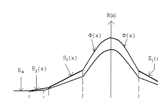
between g and f (on the right of 0), as described by Fig. 1. Since the equilibrium is symmetric, the analysis can be performed only on the right side of the city, i.e., between 0 and f. If we denote by R the agricultural land rent (outside the city),A
10
the equilibrium conditions are given by:
Land Market
[image:13.612.96.377.346.539.2]R(x)5Max
h
J1(x),J2(x),F(x),RAj
for x[f g0, f (22)Fig. 1. Urban equilibrium configuration.
10
R(x)5F(x)$J1(x) for x[[0,e[ (23)
R(x)5F(x)5J1(x) at x5e (24)
R(x)5J1(x)$F(x) for x[]e, g[ (25)
R(x)5J1(x)5J2(x) at x5g (26)
R(x)5J2(x)$J1(x) for x[] g, f [ (27)
R(x)5J2(x)5RA at x5f (28)
]
Q.m(x)1h(x)51 for x[f g0, f (29)
Constraints
e
L.M
]]
E
Lm(x) dx5 for x[f0,eg (30)2
0
g
L.M
]]
E
h(x) dx5 for x[fe, gg (31)2
e
f
U
]
E
h(x) dx5 for x[fg, fg (32)2
g
Let us comment these equilibrium conditions. The land market conditions ensure that landlords offer land to the highest bid rents, that is the CBD firms outbid workers, and outside the CBD, the employed outbid the unemployed, and the land rent market is continuous. The last three equations are the standard population constraints.
By solving (30)–(32), we easily obtain:
]
QM
]]
* *
e 5 2e 5 (33)
2
]
*
(L 1Q )M
]]]
* *
g 5 2g 5 (34)
2
] ]
N1QM
]]]
* *
f 5 2f 5 (35)
2
* *
Observe that e and f are equilibrium values that are not affected by the labor
*
]
to the number of firms, M, times their land consumption, Q. Since the city is
]
*
closed, N, the active population, is exogeneous and the city size f is thus equal to
] ]
the size of the CBD, QM, plus the size of N. Since we focus on the right size of the
*
city, we have to divide everything by 2. However, this is no longer true for g , the border between the employed and the unemployed workers, since it depends
]
* * *
crucially of the size of employment, L , and of unemployment, U 5N2L M,
that will be determined in the labor market equilibrium.
We are now able to determine the equilibrium utility and profit levels. By using Eqs. (24), (26) and (28), we easily obtain:
t ] ]
* *
z15w1 22
s
aN1LMd
2RA (36)] aN
]
*
z25b2t 2 2RA (37)
] ] 2
Q ] QM ]
] ]]
* * * * *
P 5pY 2w L1 2t2
s
aN1L Md
2t 2 2R QA (38)]
* * *
where L is the equilibrium employment level for each firm, Y] 5f(Q,L ), the
*
corresponding production level, and N5L M1U. Observe that the equilibrium
*
profit P depends (negatively) on workers’ commuting costs t because of the competition in the land market. Indeed, firms have to bid away the employed] ]
*
workers to occupy the core of the city; this is costly and equal to tQ
s
aN1L M /d
2. We will come back on this effect in the policy section.
Moreover, it is useful to identify the equilibrium space costs, i.e., land rent plus travel costs plus transaction costs (the latter is only for firms) for the employed, the unemployed and firms (identified by the subscript F) which are respectively given by:
t ] ]
* *
SC1 52
s
aN1L Md
1RA (39)] aN
]
*
SC2 5t 2 1RA (40)
]
t Q ] 2
]
* *
SCF 5 2
fs
aN1L Md
1tM 12RAg
(41)This yields the following space–cost differential between the employed and the unemployed:
*
tL M
]]
* * *
DSC 5SC1 2SC2 5 2 (42)
which will have a crucial role in the model. In fact, given that commuting costs are
*
We are now able to demonstrate thatJ1(0).J2(0). Indeed by using (36) and
*
(37), equation (21) rewrites t.e. 2tL M / 2, which is obviously always true
*
whatever the value of L .
4. The labor market equilibrium
Concerning the firms’ wage policy, we develop an efficiency wage model based on shirking (see Shapiro and Stiglitz, 1984 or Zenou and Smith, 1995). We assume that there is a moral hazard problem: workers know exactly their effort level whereas firms don’t. For simplicity, u, the effort level, takes only two discrete values: either the worker shirks,u 50 or he does not shirk andu .0. Thus, the utility of a shirker is given by:
S
*
z15z1 (43)
*
where z1 is defined by (36) and the one of a non-shirker is equal to:
NS
*
z1 5z12u (44)
We further assume that firms cannot perfectly monitor workers so that there is a probability of being detected shirking, denoted by c (firms can for example control randomly a fraction of workers). If a worker is caught shirking, he is automatically fired. In this context, firms propose to their employees a self-enforcing contract that induce workers not to shirk. This will determine the efficiency wage which is defined such that the expected utility of non-shirking is always greater than the one of shirking. We have therefore:
NS S S
*
z1 $c
f
g.z11(12g).z2g
1(12c)z1 (45)S NS
*
where z , z1] 1 and z2 are respectively defined by (43), (44) and (37), and
g 5LM /N is the probability to find a job for an unemployed worker. Thus
condition (45) means that when caught shirking (with exogeneous probability c), a worker can find another job with probabilityg, in this case he will always shirk
S NS
since z1.z1 , and can stay unemployed with probability 12g. If he does not shirk, he is sure to stay employed. In equilibrium the constraint (45) is binding so that it can be rewritten as:
u ]]]
* *
z12z2 5c(12g) (46)
which by using (36) and (37) leads to the following urban efficiency wage:
u LM
]]] ]
*
]
Then by using the fact thatg 5LM /N, we obtain:
]
u N LM
] ]]] ]
*
w1 ;w (L )1 5b1c
S
]D
1t 2 (48)N2LM
or equivalently
]
u
S D
N t ]] ] ]
*
w1 ;w (U )1 5b1 c U 12
s
N2Ud
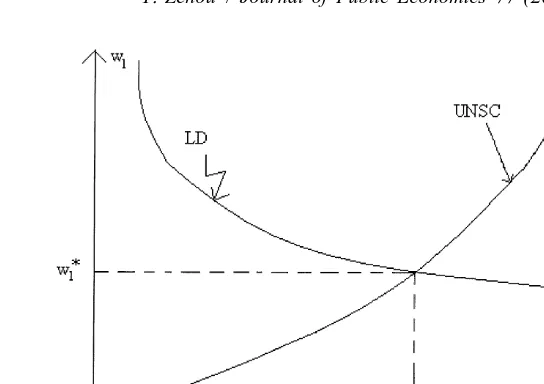
(49)Eq. (48) is referred to as the Urban Non-Shirking Condition (UNSC hereafter), i.e., the (efficiency) wage that firms must pay for each level of employment in order to induce workers not to shirk and to remain employed. The interpretation of (48) or (49) is quite intuitive. First, we obtain the standard effects of efficiency wages in a non-spatial framework. Indeed, the unemployment benefit, b, and the
*
effort level, u, affect positively w1 whereas c, the detection probability has a negative impact on it. Second, an increase in the level of unemployment, U, reduces the efficiency wage (see (49)). This captures the fact that unemployment serves as a discipline device for workers (Shapiro and Stiglitz, 1984) since when unemployment is high, workers will be reluctant to shirk because of a lower probability of finding a job if caught shirking, and thus firms can set lower efficiency wages. Last, when t, the commuting cost per unit of distance, increases firms must increase their wage in order to induce workers to remain employed. Thus, compared to non-urban efficiency wage (Shapiro-Stiglitz), the introduction of space leads to an increase of tLM / 2 in the efficiency wage. In fact, LM / 25
* *
g 2e so that firms compensate all workers by (half of) the size of the employment pool. More precisely, because of Assumption 5 (commuting costs are zero within the CBD), this means that firms compensate exactly the employed worker whose location is the furthest away from the CBD and thus residing
*
exactly at g . It is quite clear that if this individual accepts to leave welfare then all workers residing closer to firms will do the same. This means that we have a link between the location of the unemployed and labor market outcomes (‘spatial mismatch’) since the further away from jobs the unemployed are, the higher is the employed workers’ wage and the larger is the level of unemployment. Further-more, by using (42), one can see that tLM / 25 DSC, i.e., the space cost differential
between the employed and the unemployed, meaning that when they set efficiency wages, firms take into account the employed workers’ commuting costs (remember that the space cost differential between workers and non-workers is exactly equal to the commuting cost of the furthest employed worker). If for example there were no possibility of shirking (because for instance monitoring is perfect c5 1 `), then firms would set wages equal to b1tLM / 2. In this case, the worker located at
* *
commuting costs tLM / 2 (don’t forget that the employed go more often to the CBD than the unemployed and thus don’t bear the same commuting costs) so that
* *
z15z .2
To sum-up, when firms set their efficiency wage they consider three elements. The first one is b, the unemployment benefit since they must induce the unemployed to leave welfare. The second one is u/ [c(12g)] since they must induce workers not to shirk (these are the standard effects already obtained by Shapiro-Stiglitz). The third and last one, tLM / 2, is the spatial element since firms must induce their workers to remain employed. The urban efficiency wage thus has two main roles: to deter shirking and to compensate for commuting costs (see also Zenou and Smith, 1995).
Proposition 2. There is a spatial mismatch between location and labor market
outcomes since the further away from jobs the location of the unemployed is, the higher is the employed workers’ wages and the larger is the level of unemploy-ment.
Let us study how w behaves with L. By using (48), we obtain:1
2 ≠w (L )1 ≠w (L )1
]]≠L .0;]]]2 .0 (50)
≠L
lim w (L )] 1 5 1 ` (51)
L→N / M
u ]
w (L1 50)5b1 c (52)
Inequality (50) states that the efficiency wage is an increasing and convex function of employment (see Fig. 2); this is because when employment increases the threat of being fired is less important and firms must increase their wage to induce workers not to shirk. The second Eq. (51) is very important since it says that full employment is not compatible with efficiency wages. Indeed, if this were not true, then firms could always set an efficiency wage at the full employment level. In this context, workers would always shirk because even if they were caught shirking they could always find a new job. This is in contradiction with the nature of efficiency wages. Finally, Eq. (52) just states that, at zero employment level, firms set a positive (efficiency) wage.
Fig. 2. The labor market equilibrium.
The labor market equilibrium is now described. Each firm solves the following program:
* *
maxP s.t. w$w1 (53)
L
*
whereP is defined by (38). By using (38), the solution of (53) is such that:
] ]
*
w1 1tQM / 25pF9(Q,L ) (54)
which defines the labor demand curve. At this stage, it is important to observe that the labor demand curve is negatively affected by t the commuting cost (per unit of distance). Why? Because when a firm wants to hire one additional worker, the gain
]
is pF9(Q,L ) the marginal productivity of this worker. However, hiring this worker
*
will impose two costs to the firm: the wage w1 as well as the one resulting from a fiercer competition in the land market. Indeed, firms have to propose higher bids to push away more employed workers in order to occupy the central part of the city.
]
This leads to an additional cost of tQM / 2, where t is the marginal increase in land
]
rent when an additional worker is hired and QM / 2, the location of the firm which
*
] ]
*
total cost of hiring a new worker is w1 1tQM / 2 while the gain is pF9(Q,L ). Let us now state the following result.
*
Theorem 1. There exists a unique labor market equilibrium, where w1 is given
by:
]
*
u N L M
] ]]] ]]
*
w1 5b1c
S
]D
1t 2 (55)*
N2L M
*
and where L is defined by:
] ]
*
u N tL M ] tQM
] ]]] ]] * ]]
b1c
S
]D
1 2 5pF9(Q,L )2 2 (56)*
N2L M
Proof. On one hand, by (50)–(52), we know that w (L ) is an increasing and1
convex function of L, whose intercept is a positive constant (b1u/c) and has a
] ] ]
tangent at L5N /M. On the other, by Assumption 3, F9(Q,L )2tQM / 2 is
]
decreasing and convex in L (since F(.) is increasing and concave in L and tQM / 2 is the constant that does not depend on L ), and F] 9(L50)5 1 `] and limL→1`
F9(Q,L )]50 (Inada conditions). In particular, limL→1` F9(Q,L )50 means that
F9(L5N /M ) is equal to a positive constant. In this context, there exists a unique
* *
labor market equilibrium with a unique value of w1 and L (see Fig. 2). h
Observe that this theorem is contingent on the existence and uniqueness of the urban spatial configuration equilibrium (we check that below). We can now
*
examine how L varies with the different parameters. By totally differentiating
11
(56), we easily obtain:
* * *
≠L ≠L ≠L
]]≠t ,0; ]]] ,0; ]]≠M ,0
≠Q
(57)
* * *
≠L ≠L ≠L
]]≠ .0; ]],0; ]],0
c ≠u ≠b
]
* *
so that we can write L as L (t,Q,M,b,c,u). This result is quite intuitive since when the efficiency wage is positively (negatively) affected by a parameter, the
]
*
UNSC shifts leftward (rightward) so that the level of L decreases. For Q it is because the labor demand curve shifts downward when it increases. Sincet or a
does not affect the efficiency wage or the labor demand curve, it has no impact on
*
L .
We now have to check that there exists a unique urban equilibrium as described by Fig. 1. By plugging (48) in (36)–(38), we obtain:
] ]
11
* *
] ]
atN u N
]] ] ]]]
*
z15b2 2 1c
S
]D
2RA (58)*
N2L M
] atN
]]
*
z25b2 2 2RA (59)
] ] 2
u N QM
] ] ]]] ]]
* * *
P 5p.f(Q,L )2
F S
b1 ]DG
L 2tc N2L M* 2
t ]] ] ]
] * *
22
f
aNQ1L M Ls
1Qdg
2R QA (60)]
* *
where L is defined by (56) and can thus be written as L (t,Q,M,b,c,u). It is easy
* *
to verify that in equilibrium, z1 .z , i.e., the employed are better off than the2
unemployed, since
]
u u N
]]] ] ]]]
* *
z12z2 5c(12g)5c
S
]D
(61)*
N2L M
which is the surplus for the employed workers. Moreover, we assume that b and p
* *
are large enough so that z2 andP are always strictly positive. We have also:
]
*
(L 1Q )M
]]]
* *
g 5 2g 5 (62)
2
*
where L is defined by (56). In this context, by using (58)–(60), and (17), (18), (12) and (33), the equilibrium land rent is given by:
2 2
M x
]
] ]
* * *
t
s
aN1L M / 2d
1tS
2]2D
1RA for x[f2e ,e g
4 Q] ] ]
* * *
t (L
f
1Q )M1a(N1QM )22(11a) x / 2u ug
for x[f2g ,2e g
1R and x * *[fe , g g
A
*
R (x)5
] ]* *
at
fs
N1QMd
22 xu ug
/ 21RA for x[f2f ,2g g* *
and x[fg , f g
R for x *[]2`,2f ]
A
*
and x[[ f ,1`[
(63)
Theorem 2. The monocentric city is an equilibrium configuration if the following
condition holds:
tM
]]]
t# ];D2 (64)
2(11a)Q
Proof. First, if condition (24) is satisfied, then condition (25) can be replaced by:
* 9 *
F 9(e ),J1(e ) (65)
which, by using the equilibrium land rent, is equivalent to:
tM
]]]
t, ];D1 (66)
(11a)Q
In the same way, if condition (26) is satisfied, then condition (27) can be replaced by:
9 * 9 *
J1( g ),J2( g ) (67)
which is always true by Proposition 1.
We must now check that (23) is verified. If condition (24) is satisfied then,
*
because of the strict concavity ofF(x) in the interval 0,e , (23) can be replacedf g by (using the equilibrium land rent):
F(0)$J1(0) (68)
which is equivalent to (64). Notice that if condition (64) is verified then (66) is also satisfied since D2,D .1 h
The following comments are in order. First, the endogeneous formation of a monocentric city is possible only if workers’ commuting cost t (per unit of distance) is low and firms’ transaction costt(per unit of distance) is large. This is quite intuitive since the transaction cost is the agglomeration force to the CBD for firms (viatT(x)), and the commuting cost is the dispersion force for firms (via the
efficiency wage) and the attraction force for workers. Thus in order to have a monocentric city it must be that firms bid away workers from the CBD so that the
]
agglomeration force dominates the dispersion force. Second, the increase of Q,
]
5. Transportation policies
In this section, we want to analyze the importance of commuting costs in our framework and derive some transportation policy implications that fight against the negative link between the location of the unemployed and labor market outcomes. However, the role of commuting costs in this model is quite complex because of the interaction between land and labor markets. We would like here to emphasize the main mechanisms at work when commuting costs vary.
First, when t varies, it modifies the Urban Non Shirking Condition (UNSC) curve through its effect on the space–cost differential. If, for example, t decreases, then the UNSC curve shifts downward (or rightward) so that, for any given employment level L, wages are lower compared to the initial situation. This is because the space–cost differential decreases and thus firms, who want to induce workers to stay employed, have to compensate less their workers in terms of commuting costs. This is what we call the compensation effect.
Second, when t varies, it affects the labor demand curve since the cost of an additional worker is modified because of changes in the intensity of competition in the land market. More precisely, when commuting are lower, the attraction to the city-center is weaker since it is less costly to go there and thus competition for central location is less intense so that land prices decrease. Therefore, when t decreases, the labor demand curve shifts upward (or rightward) so that, for any given wage level, employment is higher compared to the initial case. The explanation is that, when a firm hires an additional worker, its marginal cost is lower than before because of a weaker competition in the land market. This is referred to as the spatial effect.
Third, the net effect of this variation is the following. When t is reduced, the UNSC curve shifts downward and the labor demand curve shifts upward. Thus, employment unambiguously rises but wages can either increase or decrease depending of the slopes of these two curves.
The main message of this analysis is that both land and labor markets interact. This suggests that a policy subsidizing commuting costs affects both land and labor markets and the resulting impact could be surprising. We would therefore like to analyze a policy that subsidizes the commuting costs of all workers and compare it with a policy that only targets the unemployed. We will compare these two policies with our initial model (without subsidy), which is referred to as the ‘base case’. In order to keep things simple, we do not consider the government’s budget constraint so that unemployment benefits and commuting cost subsidies are
12
exogeneously financed.
12
13
5.1. Subsidizing all commuting costs
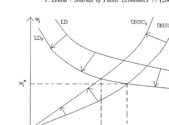
Let us start with a policy that subsidizes all workers’ commuting costs (both employed and unemployed workers), where 0,d ,1 is the ad valorem subsidy paid by the (local) government. As discussed in the introduction, the aim of this policy is to improve the city transportation network since there is a link between the location of the unemployed and the unemployment level (see Proposition 2). Basically, commuting costs per unit of distance are reduced for all workers who now support just a part of it, i.e. (12d)t. As above, we decompose the effect of the reduction in commuting costs in two parts: the effect on the UNSC curve and
14
the effect on the labor demand curve. By using (42), it is easily verified that:
LM LM
] ]
* *
DSCd 5(12d)t 2 5 DSC 2d.t 2 (69) which means that the space–cost differential between the employed and the unemployed workers is reduced compared to the base case. This implies that the UNSC shifts downward since firms need to compensate less their workers who are now ‘richer’ (their commuting costs are lower). Moreover, subsidizing commuting costs for all workers shifts the labor demand curve upward since the marginal cost of employment is lower than in the base case. Indeed, the labor demand curve is now defined by:
]
(12d)tQM ]
]]]]
w11 2 5pF9(Q,L )
]
so that the gain of employing an additional worker is still pF] 9(Q,L ) but the cost is lower and equal to w11(12d)tQM / 2. This is due to the fact that, when firms wants to hire an additional worker, the competition in the land market becomes less intensive (compared to the base case) since commuting costs are lower. The net effect, described in Fig. 3, leads to an increase of employment and thus a reduction in unemployment but has an ambiguous effect on efficiency wages. More precisely, we have:
] *
L M
u N d
] ]]] ]]
* *
w1,d5b1c
S
]D
1(12d)t 2 _w1*
N2L Md
so that two effects are present for wages when commuting costs are subsidized. The shirking effect is positive since, when t decreases, unemployment decreases so that firms have to increase their wage because the threat of unemployment is less
13
Throughout this section, we assume that the equilibrium condition (64), which is now defined by ]
(12d)t#tM / 2(11a)Q, always holds. 14
Fig. 3. The impact of subsidizing all commuting costs on the labor market.
severe (unemployment acts as a ‘worker discipline device’). The compensation
effect captured by the space–cost differential, already mentioned above, is
ambiguous since when commuting costs are subsidized, firms have to compensate
* *
more workers (Ld .L ) but at a lower price t.
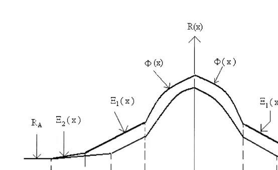
In the land market, it is clear that competition is weaker so that the equilibrium
* * *
land rent R (x) defined by (63) decreases for all x[f2f , f g. This is illustrated
*
by Fig. 4 where gd is the border between the employed and the unemployed when
* *
commuting costs are subsidized for all workers (with gd .g since employment is higher).
Moreover, equilibrium utilities, inequality and profit are given by:
] ]
a(12d)tN u N
]]]] ] ]]]
* *
z1,d5b2 2 1c
S
]D
2RA.z1 (70)*
N2L Md
] a(12d)tN
]]]]
* *
z2,d5b2 2 2RA.z2 (71)
] ]
u N u N
] ]]] ] ]]]
* * * * * *
Dzd ;z1,d2z2,d5
S
]D
. Dz ;z1 2z2 5S
]D
c N2L M*d c N2L M*
Fig. 4. The impact of subsidizing all commuting costs on the land market.
] ] 2
u N QM
] ] ]]] ]]
* * *
P 5d p f(Q,L )d 2
F S
b1 ]DG
L 2tc N2L M*d 2
(12d)t ]] ] ]
]]] * *
2 2
f
aNQ1L M Lds
d 1Qdg
2R QA _P* (73) The following comments are in order. First, the employed workers are better off when commuting costs are subsidized (see (70)). Indeed, even though their equilibrium wage can either be higher or lower, they have lower land rents and commuting costs (see Fig. 4) and a higher wage premium due to the shirking effect so that the net effect is positive. Second, this policy also increases the well being of the unemployed (see (71)). This is a pure spatial effect since their land rents and their commuting costs are reduced (see Fig. 4). Third, inequality, as measured by the utility difference, rises (see (72)) because there is less unemployment threat. Note that the utility difference is measured only by the shirking element of the efficiency wage, since, by definition, the other elements of the efficiency wage (unemployment benefits and space–cost differential) are set such that utilities between the unemployed and the employed workers are equal. Finally, the effect on the equilibrium profit is ambiguous since, on one hand, there is less competition in the land market but, on the other, firms employ more people at a higher cost. Observe that, if we take the variance of utilities to measure inequality (which takes into account the distribution of all workers; see e.g. Cowell, 1995), we obtain exactly the same result. Indeed, if we define inequality in the base case by the following equation (variance):]
* *
L M ] N2L M ]
2
S
D
2]] ]]]
* * *
where
]
* *
L M N2L M
] ]] *
S
]]]D
*z5 N z1 1 N z2
is the average utility, then it is easily verified that:
* *
Id .I
*
where Id is the inequality (defined in terms of variance) when the commuting costs of all workers are subsidized. The interesting feature here is that the change in variance takes into account the change in the composition of the population of workers after the policy.
*
If we now define the equilibrium workers’ surplus Sd as the weighted sum of
15
utilities , i.e.,
]
* * * * *
Sd ;Ld z1 1
s
N2Ldd
z2then, it can easily be shown that:
* *
Sd .S
*
where S is the workers’ surplus in the base case. The following proposition summarizes our findings.
Proposition 3. When commuting costs of all workers are subsidized, all workers
are better off, the workers’ surplus increases and unemployment is reduced.
However, inequality increases and firms’ profits can either increase or decrease.
16
5.2. Subsidizing only the unemployed workers’ commuting costs
Let us now focus on the second policy where the government supports transportation only for the unemployed (by subsidizing only the unemployed workers’ commuting costs) so that the employed and unemployed workers’ commuting costs are respectively equal to t15t and t25(12s)t, where 0,s,1 is the ad valorem subsidy. The aim of this policy is do reduce the ‘spatial mismatch’ between the location of the unemployed and the unemployment level (Proposition 2) by reducing the distance between the location of the unemployed and jobs (since it is less costly to go to the CBD).
Contrary to the previous policy, we have to undertake part of the analysis again
15
In order to focus on workers’ utilities only, we do not include the utility of absentee landlords in the definition of the surplus as well as firms’ rights.
16
since this policy introduces an asymmetry between the employed and the
17
unemployed. Bid rents are now given by:
* *
J1,s(x)5w1 2z12(11a)t(x2e) (74)
*
J2,s(x)5b2z2 2a(12s)t(x2e) (75)
By using these values, firms’ bid rent and the land market equilibrium conditions, we easily obtain:
t ] ]
]
* * * *
z1,s5w1,s22
f
aN1L Ms 2as Ns
2L Msdg
2RA (76)] a(12s)N
]]]
*
z2,s5b2t 2 2RA (77)
] ] 2
Q ] ] QM ]
] ]]
* * * * * *
P 5s pY 2w L1 s 2t2
f
aN1L Ms 2as Ns
2L Msdg
2t 2 2R QA(78)
Let us start with the effect on the UNSC curve. For that, we have to determine the space cost differential. For the employed, the space cost is equal to:
t ] ]
]
* * *
SC1,s52
f
aN1L Ms 2as Ns
2L Msdg
1RAwhereas for the unemployed, we have:
t ]
]
*
SC2,s52
f
a(12s)Ng
1RA (79)The space–cost differential between workers and non-workers is thus given by (using (42)):
tLM LM
]] ]
* *
DSCs 5(11as) 2 5 DSC 1ast 2 (80)
This means that, compared to the base case (i.e. without subsidy), for any level of
L, the space–cost differential has increased because of the subvention. In this
context, the UNSC curve shifts upward (Fig. 5) so that, for any given employment level, wages are higher. Concerning the labor demand curve, it is easily checked using (78) that it shifts downward (Fig. 5). Indeed, the labor demand curve is defined by:
] ]
w1,s1(11a.s)tQM / 25pF9(Q,L )
17
Fig. 5. The impact of subsidizing the unemployed workers’ commuting costs on the labor market. ]
so that, when firms want to hire an additional worker, the gain is pF9(Q,L )
]
whereas the additional cost is now w11(11as)tQM / 2 (because competition in
the land market becomes fiercer compared to the base case). This means that the marginal cost of a new hiring is higher than in the base case so that, for any given wage level, firms hire less workers.
The resulting equilibrium is such that employment is always reduced and unemployment increases while the effect on wages is ambiguous. We have indeed:
]
u N LM
] ]]] ]
* *
w1,s5b1c
S
]D
1(11as)t 2 _w1 (81)N2LM
In fact, different elements are present. On the one hand, the shirking effect leads to a reduction in the efficiency wage since unemployment is more important, but, on the other, the compensation effect yields a higher efficiency wage since the space cost differential (the part that has to be compensated to the employed workers) has increased (see (80)). The net effect is thus ambiguous.
In this context, equilibrium utilities, inequality and profit are equal to:
] ]
a(12s)tN u N
]]] ] ]]]
* *
z1,s5b2 2 1c
S
]D
2RA_z1*
N2L Ms
] ]
astN uN 1 1
]] ] ]]] ]]]
* *
z1,s2z1 5 2 1 c
S
] 2]D
(82)* *
N2L Ms N2L M
] at(12s)N
]]]
* *
z2,s5b2 2 2RA.z2
where
] astN
]]
* *
z2,s2z2 5 2 (83)
]
u N
] ]]]
* * * * * *
Dzs ;z1,s2z2,s5c
S
]D
, Dz ;z1 2z2*
N2L Ms
]
u N
] ]]]
5c
S
]D
(84)*
N2L M
] ] 2
u N QM
] ] ]]] ]]
* * *
P 5s p.f(Q,L )s 2
F S
b1 ]DG
Ls 2tc N2L M* 2
s
t ]] ] ]
] * * *
22
f
aNQ1L M Lss
s 1Qdg
2R QA _Pwhere
] *
L
*
uN L
] ] s
] ]]] ]]]
* * * *
P 2 P 5s p f(Q,L )
f
s 2f(Q,L )g
1 cS
] 2]D
* *
N2L M N2L Ms
tM ] ]
] * * * *
1 2
f s
L L 1Qd
2Lss
Ls 1Qdg
(85)Our comments are the following. First, the employed workers, who do not benefit from the transportation subsidy, can incur a loss or a gain in their utility. Inspection of (82) shows that, on one hand, the compensation effect (i.e. the first term of the RHS of (82)) is such that firms have to compensate more their workers by setting higher wages, but, on the other, the shirking effect (i.e. the second term of the RHS of (82)) decreases so that firms can reduce their wages since unemployment is higher. Second, quite naturally, the unemployed utility increases since they face both lower commuting costs and land prices (Fig. 6). Third, the
18
inequality is reduced since the shirking effect is lower: firms need less to induce workers not to shirk because unemployment is higher. Finally, the effect on profit is ambiguous and can be decomposed into two parts. The first one (the first term of the RHS of (85)) is negative since production is lower when the unemployed commuting costs are subsidized (less employment leads to a lower production
18
Fig. 6. The impact of subsidizing the unemployed workers’ commuting costs on the land market.
level). The second one is positive and encompasses two effects: the shirking effect (the second term of the RHS of (85)) and the compensation / land rent effect (the third term of the RHS of (85)).
Contrary to the previous case, this policy does not always increase employed workers’ utility since, on one hand, their commuting costs and land rent are reduced (direct effect that increases their utility) but, on the other, firms must compensate the employed workers more. As we have seen below, the net effect will depend on the fact that the efficiency wage increases or decreases after this policy. Moreover, if we take the value of the workers’ surplus, then Ss_S.
Finally, it is easily verified that, compared to the base case, land rent decreases everywhere (Fig. 6) because the unemployed, who incur less commuting costs,
* *
drive down the competition in the land market. If we denote by gs ,g (since employment is lower) the border between the employed and the unemployed when commuting costs of the unemployed are subsidized, we have indeed:
2 2
M x
] ] ] ]
* * * *
t
f
aN1