U.S. Money Demand and the Welfare Cost
of Inflation in a Currency–Deposit Model
Turan G. Bali
This paper emphasizes that it is crucial to identify the proper specification of money demand as well as the appropriate monetary aggregate to find the exact welfare cost of inflation. The econometric test results obtained from the nonlinear form of money demand with Box–Cox restriction indicate that not the semi-logarithmic form but the double-log form with constant elasticity of less than one is a more accurate characterization of the actual data. The welfare cost estimates for the U.S. economy from Bailey’s (1956) consumer’s surplus and Lucas’s (1994) compensating variation approaches imply that for each monetary model (currency–deposit, single-asset) and each scale variable (income, consumption) the double-log function, compared to the constant semi-elasticity Cagan-type demand for money, yields substantial welfare gains in moving from zero inflation to the Friedman optimal deflation rate needed to bring nominal interest rates to zero. This paper also shows that the estimated welfare cost of inflation is proportional to the money stock and because M1 is about three times the monetary base in the United States, identifying M1 without modeling the distinctive roles of currency and deposits as the relevant definition of money overestimates the true welfare cost of inflation. © 2000 Elsevier Science Inc.
Keywords: Currency–Deposit Model; U.S. Money Demand; Welfare Cost of Inflation
JEL Classification: E31, E41
I. Introduction
The estimated welfare cost of inflation is proportional to the money stock, so the choice of an observed monetary aggregate to serve as “money” in the formula is crucial. Lucas (1994) chooses to use M1 as the relevant money and runs his welfare integral from a zero nominal rate to a positive rate—a procedure that lumps currency and interest-bearing
Department of Economics, Queens College, City University of New York, New York
Address correspondence to: Dr. T. G. Bali, Department of Economics, Queens College, CUNY, 65-30 Kissena Boulevard, Flushing, New York 11367-1597.
deposits together and treats this composite as non-interest bearing. In this regard, it is relevant to return to Bailey’s (1956) classic article and review his treatment of currency and deposits. Bailey used Cagan’s (1956) hyperinflation data to estimate the welfare cost of inflation. He set the real rate of interest at zero (r5 0) so that the cost of holding currency was the anticipated inflation p (a proxy for the nominal interest rate i). He assumed that competitive banks pay interest on deposits but are subject to a sterile reserve requirement. A zero-profit condition was imposed: the revenue from a bank’s interest bearing assets was completely dispersed in interest payments on deposits: id5(12m)i wheremis the required reserve ratio and i5 p in his setup. The zero-profit condition under perfect competition implies that the opportunity cost of holding deposits is (i2id) 5mi (or mp). Because deposits are partially indexed, Bailey assumed that at very high rates of inflation, the public uses only deposits and all currency would be held as bank reserves. In this case, Bailey’s welfare integrals run from zero tompto account for the partial indexing of the deposit rate to inflation. In contrast to Lucas, there is a substantial reduction in welfare cost of inflation when interest on deposits is partially indexed against inflation.
What is at issue is the polar choice of two very incomplete models. On the one hand, we can lump currency and deposits together and assume that both pay no interest. We can then run our integrals from zero to a positive interest rate. This is Lucas’ choice. On the other hand, we could assume with Bailey that all high-powered money is held as reserves and run the welfare integrals from a nominal rate of zero tomi, the opportunity cost of
holding interest bearing deposits. Lucas’ choice overstates the welfare loss of deviating from the Friedman (1969) rule. The assumption in Bailey that all deposits pay interest underestimates the welfare loss. Without a theory of banking in which the distinctive roles of currency and deposits are modeled, it remains uncertain how large is the degree of overestimation or underestimation.
As an alternative to these two polar cases, we try to model the distinctive roles of currency and deposits in Ramsey–Sidrauski infinite-horizon model. We measure the welfare cost of inflation using the traditional approach, developed by Bailey (1956), by computing the appropriate areas under currency and deposit demand curves. In our currency– deposit model, it is possible to run separate integrals: that for currency running from a zero nominal rate to a positive rate, and the integral for deposits running from zero tomi. As an alternative to Bailey’s consumer’s surplus argument, we also provide the
quadratic approximation and the square root formula, [originally developed by Lucas (1994) in a single-monetary-asset model], for evaluating the welfare loss in the currency– deposit model.
in effect, in a currency-only model because the monetary authority receives no revenue from deposits. In addition to the above-mentioned studies that deal with money demand and welfare cost analysis either in a deposits-only world or in a currency-only world, Eckstein and Leiderman (1992), Lucas (1994), and Dotsey and Ireland (1996) quantita-tively assess the welfare losses in a general equilibrium single-monetary-asset model without separating money into its currency and deposit components.
This paper extends the current literature by developing a currency– deposit model in an intertemporal optimizing framework and deriving the welfare costs of inflation in a world of both currency and demand deposits. Because currency and deposit demand functions reach a specific estimable form in the theoretical model introduced in the paper, the welfare cost function can be derived for both the consumer’s surplus approach of Bailey (1956) and the compensating variation approach of Lucas (1994). In estimating the welfare costs of deviating from a zero inflation policy and the costs of deviating from the Friedman optimal deflation rate in the currency– deposit model, the paper makes a contribution to the literature regarding the welfare costs of low inflation rates.
This study also emphasizes that the estimated welfare cost of inflation is sensitive to the specification of the money demand function and to the definition of money. Thus, it is crucial to identify the proper specification of money demand as well as the appropriate monetary aggregate to serve as “money” in the formula. To determine what form the U.S. money demand takes, the Box–Cox transformation is applied to the nominal interest rate and the proper specification of the money demand function is identified with the aid of two different econometric tests. The empirical results indicate that, for each monetary aggregate and each scale variable, the double-log function with constant elasticity is a more accurate characterization of the actual data and yields substantial welfare cost estimates for the U.S. economy compared to the constant semi-elasticity Cagan-type demand for money.
Lucas (1994), Dotsey and Ireland (1996), and Lucas (1981) use M1 to calculate the welfare cost of inflation for the American economy. As will be discussed in the paper, identifying M1 instead of the monetary base as the relevant definition of money leads to an overestimate of the true welfare loss because the estimated welfare cost of inflation is proportional to the money stock, and M1 is about three times the monetary base in the United States. Within his framework, and with his preferred constant elasticity double-log function scaled with income, Lucas (1994) finds the welfare cost of a 10 percent nominal interest rate is about 1.3 percent of GDP. In a general equilibrium monetary model, Dotsey and Ireland (1996) find the welfare cost of a sustained 4 percent inflation rate is over 1 percent of GDP when M1 is defined as money. Fischer (1981) and Lucas (1981) find the cost of inflation to be surprisingly low. Fischer computes the deadweight loss from an increase in inflation from zero to 10 percent as just 0.3 percent of GNP, identifying money with the monetary base. Lucas (1981) places the cost of a 10 percent inflation at about 0.45 percent of GNP, using M1 as the measure of money.
This paper is organized as follows. Section II describes our currency– deposit model in an intertemporal optimizing framework and outlines the microfoundations for the double-log form of money demand. Section III sets out the estimation techniques employed in money demand regression equations and provides the econometric test results for the specification of the U.S. money demand function. Section IV not only measures the costs of deviating from both a zero inflation and an optimal deflation policy but studies the sensitivity of the estimated welfare cost of inflation to the specification of money demand in both the single-monetary-asset (M1 or monetary base) model and the currency– deposit model as well. Section V concludes the paper.
II. The Currency–deposit Model
Several approaches can be found in the literature for introducing the role of money into the intertemporal optimizing framework.1To specify the distinctive roles of currency and deposits in an infinite horizon model, we modify Sidrauski’s (1967) general equilibrium single-monetary-asset model by separating M1 into its currency and demand deposit components and apply a required reserve ratio to the deposit component. In this currency– deposit model, we think about the money stock as “making life easier” because it allows people to get consumption goods without having to go to the bank and transform bonds into consumption goods all the time.
We will assume that the economy is populated by infinitely lived consumers or dynasties who derive utility from the only consumption good ctand from the real money stock, which is composed of non–interest-bearing real currency mt and interest-bearing real demand deposits dt. Each household is assumed to have access to a production function that is homogenous of degree one in its two inputs, capital and labor. We will also assume that labor is supplied inelastically so that the production function with diminishing marginal product of capital can be written as
yr5f~kt! (1)
where ytis real output, ktis real capital and dyt/dkt5f9(kt).0, d2yt/dkt25f0(kt),0. Here capital is treated as output that is not consumed, so its price is the same as that of consumption good. The households in the economy begin period t with certain amount of money and pay a lump sum tax Ht(or, if Ht, 0, receive a lump sum transfer from the
government). They can save by accumulating nominal currency Mt11 and nominal
demand deposits Dt11, by investing in real capital kt11, and by buying government bonds
Bt11. All four variables denote quantities held at the beginning of period t11. The bonds that agents buy in period t, Bt11, are sold at the nominal price zt and yield one unit of money in period t11, so that the nominal rate of return on bonds between t and t11 is it115 (12zt)/zt. The gross real rate of return on bonds is, therefore, defined as 11 rt115(11it11)/(11pt11), wherept115(Pt112Pt)/Ptis the inflation rate between
1Within the infinite horizon model, four approaches have been adopted to incorporate the role of money. The
t and t1 1. The number of bonds Bt divided by the price of the commodity Pt in that period is denoted by bt. We will assume that competitive banks pay interest on deposits but are subject to a fractional reserve requirement on demand deposits. Assuming that banks face no operating costs, the zero-profit condition under perfect competition yields
id(t)5(12mt)itimplying that the opportunity cost of holding demand deposit ismtit: the difference between it and the nominal interest on demand deposits id(t).
In each period, households have the following budget constraint
Mt111Dt111Ptkt111ztBt115Mt1Dt~11id~t!!
1Ptkt~12d!1Bt1Ptyt2Ptct2Ht (2)
in nominal terms and thus
~11pt11!mt111~11pt11!dt111kt111~11rt11! 21b
t115mt1dt~11id~t!!
1kt~12d!1bt1f~kt!2ct2ht (3)
in real terms, where ht5 Ht/Pt, andd is the depreciation rate.
We will further assume that the household preferences are time separable, that is
O
t50 `
~11r!21u~c
t,mt,dt!, (4)
where r is the subjective rate of time preference. Households maximize equation (4) subject to equation (3), and the first-order Euler conditions for the maximum problem can be written as equalities holding for each period:
uc~ct,mt,dt!2Vt50, (5a)
um~ct,mt,dt!1Vt2~11r!~11pt!Vt2150, (5b)
ud~ct,mt,dt!1~11id~t!!Vt2~11r!~11pt!Vt2150, (5c)
Vt2~11r!~11rt!21Vt2150, (5d)
Vt~11f9~kt!2d!2~11r!Vt2150, (5e)
whereVt andVt21are the Lagrangian multipliers attached to the budget constraints at
time t and t 2 1, respectively. From equations (5d) and (5e), we have VVt21
t
5 ~11rt! ~11r! 5
~11f9~kt!2d!
~11r! , which implies that the real rate of return on capital equals
the real rate of interest on bonds: (f9(kt)2d)5rt. Dividing equations (5b) and (5c) by
equation (5a), and using the fact thatVt21
Vt
5 ~11rt!
~11r! where (11rt)5 11it 11pt
, we get
the following conditions:
um~ct,mt,dt! uc~ct,mt,dt!
5211~11r!~11pt! Vt21
ud~ct,mt,dt! uc~ct,mt,dt!
521~11id!1~11r!~11pt! Vt21
Vt 5it2id~t!, (6b)
which imply
um~ct,mt,dt!5ituc~ct,mt,dt!, (7a)
ud~ct,mt,dt!5~it2id~t!!uc~ct,mt,dt!. (7b)
In order to find a closed from solution for real currency and real deposit demand functions, suppose that the period utility function takes the following CES-isoelastic form:
u~ct,mt,dt!5 $@g11/u
ct
~u21!/u1g 2 1/u
mt
~u21!/u1g 3 1/u
dt
~u21!/u#u/~u21!%121
s
121
s
. (8)
whereu. 0 is the intertemporal substitution elasticity. Imposing CES-isoelastic prefer-ences on first-order conditions, equations (5a), (5b), and (5c), yields a generalization of asset demand functions that take the following double-log form with constant elasticity of
u:
mt5
S
g2
g1
D
it
2u
ct (9a)
dt5
S
g3
g1
D
~it2id~t!!2uct (9b)
where the consumption elasticities of demand for real currency and real deposits equal one.2
2Imposing the same interest rate elasticity on currency and deposit demand may seem too restrictive to the
reader. However, in this paper, a currency–deposit model is developed to estimate the “steady-state” welfare cost of inflation and the welfare cost analysis is compatible with a steady state only if the velocity of money remains constant. In turn, constant velocity requires a unitary scale elasticity of demand for money. Therefore, it is crucial that the scale elasticity is unity. If this were not the case, we could not use steady-state analysis. The use of unitary scale elasticity in our theoretical model leads currency and deposit demand functions to have the same elasticity or semi-elasticity with respect to their own opportunity costs. To illustrate this, instead of using the CES-isoelastic utility function given in equation (8), we can employ its more flexible version,
u~ct,mt,dt!5
S
1 12vDFS
1 12g
D
~ct12g21!1
S
w12a
D
~mt12a21!1
S
f12b
D
~dt12b21!
G
121v, in our intertemporal optimizing framework, which yields the following double-log currency and deposit demand functions:
mt5w1/ait
21/ac
t
g/a, (9a9)
dt5f1/b~it2id~t!!21/bct
g/b, (9b9)
The monetary model developed in this section is quite new in the sense that it yields a specific estimable form for asset demand functions as in equations (9a) and (9b), which are used to derive the welfare cost function in a currency– deposit framework for both the consumer surplus and the compensating variation approaches. In addition, the currency– deposit model is more general than the earlier monetary models because, as discussed in the previous section, it nests the currency-only and deposits-only models.
As presented above, standard utility functions yield double-log demands for money although the semi-log form has been widely used in money demand studies, more a matter of convenience than theoretical or empirical attractiveness. The convenience comes from its simplicity, the fact that steady-state seigniorage is easily defined at a constant nominal interest rate and the fact that the seigniorage-maximizing interest rate as well as the maximum seigniorage are easily derived. However, the semi-logarithmic form has its drawbacks. The micro-foundation of the semi-log specification in either “the shopping time” or “the money-in-the-utility function” approach is somewhat ad hoc. We have to impose a specific form on the utility function or on the shopping time technology in order to arrive at the constant semi-elasticity Cagan-type demand for money. The utility function and the similarly shaped shopping time technology take the following unusual forms, respectively:
u~ct,mt,dt!5
mt~11w 2ln mt!
a 1
dt~11v 2ln dt!
b 1v~ct!,
um.0,ud.0,uc.0
c~ct,mt,dt!5
mt~ln mt2w 21t!
a 1
dt~ln dt2v 21t!
b 1v~ct!,
cm,0,cd,0,cc.0
which imply the following Cagan-type demand for currency and deposits:
ln mt5w 2 avcit,
ln dt5v 2 bvc~it2id~t!!,
where the marginal utility of consumption is assumed to be a positive constant, vc.0.
III. The Specification of the Money Demand Function
This section concentrates on the econometric approach we use to identify the proper specification of U.S. money demand. A search for an improved specification of the long-run demand for money leads us to consider econometric issues in the treatment of short-run dynamics. The calculation of the parameters of long-run relationships from estimated models, and the forms of particular models, such as partial adjustment and error
correction models, are also discussed in this section.
To determine what form the U.S. money demand will take, the Box–Cox
transforma-tion,
g~l!~i
t!5 itl21
is applied to the itvariable. Note that in the following regression equation, which assumes a unitary quantity elasticity of money demand,
ln~mt/qt!d5b01b1
S
itl21
l
D
1et, (11)when lequals one, equation (11) reduces to
ln~mt/qt!d5~b02b1!1b1it1et, (12)
and the demand for real money balances becomes semi-logarithmic in it. Whenlequals zero, the transformation is, by L’Hopital’s rule,
liml30
S
it l
21
l
D
5ln itHence, l50 in g(l)(i
t) implies that the demand for real balances is logarithmic in it,
ln~mt/qt!d5b01b1ln it1et. (13)
In estimating the regression equation of the demand for real balances, the crucial step is to define the specific form of money demand and to find an efficient mechanism to estimate short-run money demand equations, which are consistent with imposed long-run relationships. The partial adjustment and error correction models have been widely used as short-run dynamic specification to estimate long-run parameters of money demand. In this paper, dynamics are first allowed for by means of real partial adjustment model along the lines of Hwang (1985), who rationalizes partial stock adjustment as an optimization between costs of adjustment of money balances and costs of being out of equilibrium:3
ln mt2ln mt215f~ln mt d2
ln mt21!. (14)
Substituting equation (12) into equation (14) yields
ln~mt/qt!d5~fb0!1~fb1!
S
itl21
l
D
1~12f!ln~mt21/qt21!1 «t. (15)As an alternative to the partial adjustment model, a general distributed lag model and its transformation to error correction have been increasingly used for estimation of money demand. Following Baba et al. (1992) and Banerjee at al. (1993) among many others,4we apply the error correction mechanism to U.S. money demand. To illustrate the derivation
3Partial adjustment is typically motivated by cost-minimizing behavior wherein the costs of disequilibrium
are balanced against adjustment costs. Following Hwang (1985), consider a quadratic cost function of the form:
C5Ã1@ln Mtd2ln Mt]21Ã2[(ln Mt2ln Mt21)2z(ln Pt2ln Pt21)]2
where the first and second terms of the function correspond to the disequilibrium and adjustment costs, respectively. Minimizing costs with respect to Mtyields:
ln Mt2ln Mt215f(ln Mtd2ln Mt21)1z(12f)(ln Pt2ln Pt21)
wheref5Ã1/(Ã11Ã2). Thus, whenz51, this expression reduces to the real partial adjustment model in
which real balances are adjusted: ln mt2ln mt215f(ln mt d2ln m
t21).
4For example, Hendry (1980) used this procedure for U.K. money demand and Rose (1985) estimated an
of this model from a distributed lag model, we consider a specification with only one lag of each variable as in
ln~m/q!t5a01a1it1a2it211a3ln~m/q!t211et (16)
for the semi-log form with unitary quantity elasticity. Note that the long-run interest rate semi-elasticity in this model is (a11 a2)/(12a3). Now subtract ln (m/q)t21from both sides of equation (16) and then add and subtracta1it21on the right hand side to get
Dln~m/q!t5a01a1Dit1~a11a2!it211~a321!ln~m/q!t211et. (17)
To estimate the error correction model, equation (17) can be rewritten as
Dln~m/q!t5a01a1Dit1~a321!@ln~m/q!t212kit21#1et, (18)
wherek5(a11a2)/(a321). Equation (18) is called an error correction model because the term [ln (m/q)t212kit21] represents last period’s error or deviation of money from its long-run relationship with interest rate.
To determine whether the money demand function with the error correction mechanism is logarithmic or semi-logarithmic, the Box–Cox transformation is applied to itand it-1in equation (16):
ln~m/q!t5a01a1
S
itl1
21
l1
D
1a2
S
it21 l2
21
l2
D
1a3ln~m/q!t211et. (19)
Note that when l15 l25 0, equation (19) reduces to the error correction model with double-log function
Dln~m/q!t5a01a1Dln it1~a321!@ln~m/q!t212kln it21#1et. (20)
Whenl15l251, the demand for real balances takes the semi-logarithmic form given in equation (18).
Having provided the framework we utilize to identify the true form of U.S. money demand, we now describe the data, and then present the money demand estimates and econometric test results.
After all variables used in our analysis are seasonally adjusted by the standard U.S. Bureau of Census methods of seasonal adjustment, the demand for real balances is estimated with four different monetary aggregates (currency, demand deposits, monetary base, M1), using quarterly data for the period 1957:I–1997:II.5 Furthermore, to test whether the empirical results depend on the choice of a scale variable, two different quantity variables (consumption, income) are utilized in money demand estimates. We use the GDP deflator when real GDP and the consumer price index (CPI) when real consumption is employed as the scale variable. The 3-month T-bill rate is used as the opportunity cost of holding money in our estimation.
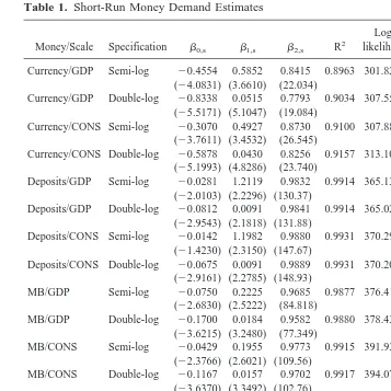
The demand for real balances is estimated by means of OLS when the short-run partial adjustment specification takes either the semi-log form: ln (m/q)t 5b01b1it 1b3ln (m/q)t21, or the double-log form: ln (m/q)t 5b01b1ln it1 b3ln (m/q)t21. The OLS estimates and related statistics of the partial adjustment model are presented in Table 1. When dynamics are allowed for by means of autoregressive distributed lag model, OLS
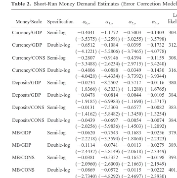
is applied both to the error correction model with the semi-log function:Dln (m/q)
t5a0
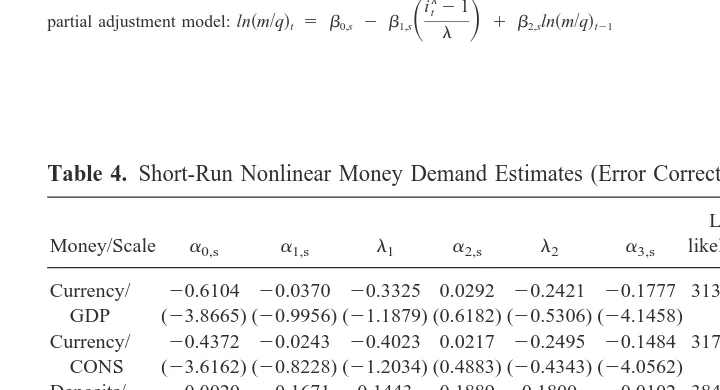
1a1Dit1(a11a2) it211(a321) ln (m/q)t211et, and the model with the double-log function:Dln (m/q)t5a01a1Dln it1(a11a2) ln it211(a321) ln (m/q)t211et. Table 2 shows the short-run estimates and related statistics of the error correction model. The nonlinear money demand estimates with the partial adjustment and error correction models are demonstrated in Tables 3 and 4, respectively.6 The long-run values of the
6Although they are not presented in our tables, the statistical results from the augmented Dickey–Fuller
(1979) test imply that all of the variables used in this study are characterized as nonstationary I(1) variables because we find that there is a unit root in the level of the variables but there is none in their first differences. Because the variables are found to be nonstationary I(1), we check for cointegration using Engle–Granger (1987)
Table 1. Short-Run Money Demand Estimates
Money/Scale Specification b0,s b1,s b2,s R2
Log-Note: This table presents the short run estimates of the demand for currency, deposits, monetary base (MB), and M1 using quarterly data for the period 1957:I and 1997:II. The scale elasticity of money demand is assumed to be unity.b’s are the coefficients in the semi-log and double-log form of money demand with the partial adjustment model. t-ratios are shown in parentheses. *(**) indicate the cases in which the h statistics and ARCH(1)-statistics are significant at the 5 percent (1 percent) level of significance. The short-run parameters are estimated from the following semi-log and double-log specification with the partial adjustment model: ln (m/q)t5b0,s2b1,sit1b2,sln (m/q)t21(semi-log), ln (m/q)t5b0,s2b1,sln it1b2,sln (m/q)t21
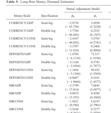
parameters presented in Table 5 are unscrambled from the short-run estimates given in Tables 1 and 2.
As pointed out earlier, this section attempts to identify the correct specification of the U.S. money demand function employing the nonlinear form of money demand with
test. According to the cointegration test results, the U.S. time series are cointegrated of order (1,1). We test autocorrelation using the Durbin-h statistics. As presented in Tables 1 through 4, there is autocorrelation in some of the estimated money demand equations when consumption is used as the scale variable. Given the presence of a lagged endogenous variable, autocorrelation implies that OLS estimates are biased and inconsistent. We test for the presence of autoregressive conditional heteroscedasticity using ARCH-LM test. As shown in Tables 1 through 4, there are no ARCH errors in the estimated money demand equations (except for the deposit demand scaled with consumption) at the 1 percent level of significance.
Table 2. Short-Run Money Demand Estimates (Error Correction Model)
Money/Scale Specification a0,s a1,s a2,s a3,s
Table 3. Short-Run Nonlinear Money Demand Estimates (Partial Adjustment Model)
Note: This table presents the nonlinear short run estimates of the demand for currency, deposits, monetary base (MB), and M1 using quarterly data for the period 1957:I and 1997:II. The scale elasticity of money demand is assumed to be unity. t-ratios are shown in parentheses. *(**) indicate the cases in which the h statistics and ARCH(1)-statistics are significant at the 5 percent (1 percent) level of significance. The short-run parameters are estimated from the following nonlinear specification with the
partial adjustment model:ln~m/q!t 5 b0,s2 b1,s
S
itl
21
l
D
1 b2,sln~m/q!t21Table 4. Short-Run Nonlinear Money Demand Estimates (Error Correction Model)
Money/Scale a0,s a1,s l1 a2,s l2 a3,s
Note: This table presents the nonlinear short run estimates of the demand for currency, deposits, monetary base (MB), and M1 using quarterly data for the period 1957:I and 1997:II. The scale elasticity of money demand is assumed to be unity. t-ratios are shown parentheses. *(**) indicate the cases in which the h statistics and ARCH(1)-statistics are significant at the 5 percent (1 percent) level of significance. The short-run parameters are estimated from the following nonlinear specification with the error
Box–Cox restriction: a semi-logarithmic Cagan-type money demand function will be the proper specification if the value ofl in equation (15) or if the values of l1 andl2 in equation (19) are found to be statistically not different from one whereas iflin the partial adjustment model orl1andl2in the error correction model are statistically equal to zero then the demand for real balances is logarithmic in it. In other words, having computed the estimate ofl(orl1andl2), the next step is to test whether the truel(or truel1andl2) is (are) statistically different from one or different from zero. To serve the purpose, two different econometric tests—the Wald test and the Likelihood Ratio test—are applied to the nonlinear money demand equations presented in equations (15) and (19). As demon-strated in Tables 6 and 7, for each monetary aggregate and each scale variable, the semi-log form is rejected but the double-log form is not at the 5 percent level of
Table 5. Long-Run Money Demand Estimates
Money/Scale Specification
Partial Adjustment Model Error Correction Model
b0 b1 a0 a1 Note: This table presents the long-run parameter estimates of the demand for currency, deposits, monetary base (MB), and M1 with the partial adjustment and error correction models. The long-run parameters are unscrambled from the short-run estimates:b05b0,s/(12b2,s) andb15b1,s/(12b2,s) are obtained from ln (m/q)t5b0,s2b1,sit1b2,sln (m/q)t21or ln (m/q)t
5b0,s2b1,sln it1b2,sln (m/q)t21a05 2a0,s/a3,sanda15 2a2,s/a3,sare obtained fromDln mt5a0,s1a1,sDit1a2,s
significance, implying that the double-log function with constant elasticity of less than one is a more accurate characterization of the actual data.
IV. The Welfare Cost of Inflation
In the theoretical literature, it is a widely accepted idea that seigniorage is a certain amount of revenue a government collects, with the aid of its central bank, from the issue of monetary base. Seigniorage can be viewed as a tax on private agents’ domestic currency holdings because money creation causes inflation, thereby lowering the real value of nominal assets. Inflation imposes a tax on money holdings because it is the rate at which individuals lose the purchasing power of a dollar. Therefore, individuals change their holdings and their use of money to lower the total cost of holding money when inflation rises. Their efforts to do so, however, reduce total services from real money balances, thereby lowering individuals’ welfare. This loss is the welfare cost of inflation.
Table 6. Testing the Proper Specification of Money Demand (Partial Adjustment Model)
Wald Test Wald Test LR Test LR Test
Money/Scale Semi-log Double-log Semi-log Double-log
Currency/GDP 27.703 3.7564 15.172 3.7040
Currency/CONS 24.053 3.7765 14.238 3.7924
Deposits/GDP* 0.0271 0.2717 0.0130 0.2212
Deposits/CONS* 0.0524 0.2287 0.0040 0.1692
MB/GDP 12.795 2.4522 6.2358 2.1856
MB/CONS 12.338 2.5226 6.7020 2.4152
M1/GDP 8.4344 0.9263 4.1316 0.8360
M1/CONS 7.0691 0.8520 3.8862 0.8218
Note: This table presents the Wald and Likelihood Ratio (LR) test statistics for determining the correct specification of U.S. money demand estimated with the partial adjustment model. For each monetary aggregate and each scale variable, the semi-logarithmic form is rejected but the double-log form is not at the 5 percent level of significance since the critical value is
x(1,0.05)53.84.
*The semi-logarithmic form is not rejected when money is identified with demand deposits.
Table 7. Testing the Proper Specification of Money Demand (Error Correction Model)
Wald Test Wald Test LR Test LR Test
Money/Scale Semi-log Double-log Semi-log Double-log
Currency/GDP 25.919 1.898 20.512 2.515
Currency/CONS 21.210 2.183 18.246 3.097
Deposits/GDP 12.001 0.465 7.954 0.520
Deposits/CONS* 5.478 1.345 3.298 1.733
MB/GDP 29.016 2.302 23.151 3.596
MB/CONS 22.027 2.144 18.859 3.685
M1/GDP 15.168 0.419 10.428 0.456
M1/CONS 9.225 0.777 6.634 0.842
Note: This table presents the Wald and Likelihood Ratio (LR) test statistics for determining the correct specification of U.S. money demand estimated with the error correction model. For each monetary aggregate and each scale variable, the semi-logarithmic form is rejected but the double-log form is not at the 5 percent level of significance since the critical value isx(2,0.05) 55.99.
In this section, we attempt to quantify the welfare loss of deviating from a zero inflation policy and answer the question: How much welfare does the United States gain in moving from zero inflation to the Friedman optimal deflation rate needed to bring nominal interest rates to zero? We also measure the sensitivity of the estimated welfare cost of inflation to the specification of money demand and to the definition of money in both the currency– deposit model and the single-monetary-asset model.
We first use the quadratic approximation (for the semi-log function) and the square root formula (for the double-log function), originally introduced by Lucas (1994) in a single-monetary-asset model, then the consumer’s surplus approach of Bailey (1956). Bailey’s original study uses the constant semi-elasticity Cagan-type demand for money, and as will be demonstrated in this section, the semi-log function yields a quadratic formula for the welfare loss. In this case, the welfare cost of inflation increases with the square of the interest rate, assigning large costs to very high rates of inflation but trivial costs to moderate inflation’s. That is, with the semi-logarithmic form, the objective of a zero inflation rate has negligible benefit, and an additional gain in moving from a zero inflation rate to a zero nominal interest rate that would attain the Friedman (1969) optimum is assigned an even smaller value. We will also provide a square root formula for the welfare cost of inflation as an alternative to Bailey’s consumer’s surplus argument that uses the appropriate area under a semi-log money demand function as an estimator of the welfare cost of inflation.
Lucas compares two economies with the same preferences and technology, both in a deterministic steady state with constant rates of money growth and price inflation, and constant nominal interest rates equal to the common real rate plus the inflation rate. He assumes that in one economy monetary policy induces a steady deflation at the Friedman optimal rate corresponding to a nominal interest rate of zero; while in the other money grows so as to induce a positive nominal interest rate. In this setting, the welfare cost of inflation is defined as the fraction of income people would be willing to forego to move from the second economy to the first.
Following Lucas, we will now assume that each household in the model described in section II is endowed with one unit of time, which is inelastically supplied to the market and which produces yt5y0(1 1 F)
t
units of the consumption good in period t. Hence one equilibrium condition is ct 5 yt 5 y0(1 1 F)
t
. Now consider a balanced growth equilibrium in which the money growth rate is constant atj5(Mt112Mt)/Mt, so that the inflation factor (11 p) is constant at the value (1 1 j)/(11F), the real currency-real income ratio mt/yt5mt/ctis constant at m#, and the real deposit-real income ratio dt/yt5 dt/ctis constant at d#. In this case, equations (7a) and (7b) become:
um~1,m#,d#!5iuc~1,m#,d#! (21a)
ud~1,m,d#!5~i2id!uc~1,m#,d#! (21b)
household in the steady state is u (1, m#(i), d# (mi)).7Provided that m#9(i) [5m#(i)/(i)],
0 and d#9(mi) [5 d# (mi)/(i)] , 0, this utility is maximized over nonnegative nominal interest rates at i50: the Friedman rule of a deflation equal to the real rate of interest. We define the welfare cost w(i) of a nominal rate of interest i to be the percentage income compensation needed to leave the household indifferent between i and 0. That is,
w(i) is defined as the solution to:
u@11w~1!,m#~i!,d#~mi!#5u@1,m#~0!,d#~0!#. (22)
Our objective is to use an estimated m#(i) and d#(mi) to obtain a quantitative estimate of the
function w(i). One way to do this is to take the second-order Taylor series expansion of the function w(i) about the zero nominal interest rate. The first two derivatives of w(i) are found by using equations (21a), (21b), and (22). Total differentiation of (22) gives:
uc w9(i) 1 um m#9(i) 1 udmd#9(mi) 5 0, which can be written as: w9(i) 52 um
uc m#9~i!
2 ud uc
md#9~mi! 5 2im9~i! 2 im2d#9~mi!sinceum
uc
5 i from equation (21a) andud uc
5(i2
id)5mi from equation (21b). Then we find the second derivative of w(i) with respect to i: w0(i)5 2m#9(i)2im#0(i)2 m2[d#9(mi)1imd0(mi)]. Thus, the Taylor series expansion
of the function w(i) about i50 gives
w~i!5w~i!ui501w9~i!ui50~i20!1 1
2w0~i!ui50~i20!2
51
2i
2@2m#9~0!2m2d#9~0!# (23)
because w(i)ui505w9(i)ui5050 and w0(i)ui505 2m#9(0)2m 2
d#9(0). To quantify the right side of equation (23) for the semi-log function used by Cagan (1956) and Bailey (1956),
we will use estimates of the semi-elasticity 1
m#~i!m#9~i! 5
1
d#~mi! d#9~mi! 5 2hassuming
that the demand for currency and deposits have the same semi-elasticity. In terms ofh, equation (23) can be written as:8
w~i!51
2hi 2@m
#~0!1m2d#~0!# (24)
where m#(0) and d#(0) are the inverses of the annual income velocities of currency and deposits at i 5 0, respectively, assuming that i is an annual nominal interest rate and income is normalized at unity.
7The general solution for m
# and d#from equations (21) implies that both are functions of both interest rates
i and id. But, the zero-profit condition, id5(12m)i, under perfect competition implies that m# and d# are functions of i andmi, respectively.
8Assuming different semi-elasticities for currency and deposit demand schedules, 1
m#~i!m#9~i! 5 2h for currency and 1
d#~mi!d#9~mi! 5 2«for deposits, the welfare cost of inflation for the semi-log function in the currency–deposit model can be written as:w~i! 5 1
2i
2@hm
To obtain an explicit form of w(i), we need an estimate of the semi-elasticity (h). Here and below, we will use the parameter estimates obtained from 1957:I–1997:II quarterly U.S. time series. We will now illustrate the procedure for finding a general formula for the semi-log function in the currency– deposit model. Assuming that the functions m#(i) and
d#(mi) pass through the points (m0, i0)5(0.0509, 0.0520) and (d0,m0i0)5(0.1034, 0.0042) observed in 1997:II and using the constant semi-elasticity9h57.8365 (a1in footnote 8), we obtain the estimate m#(0)5(0.0509)e(7.8365)(0.0520)50.0765 because m#(i)5m#(0) e2hi, and d#(0)5 (0.1034)e(7.8365)(0.0042)5 0.1074 because d#(mi)5 d#(0) e2h(mi).
Hence, from equation (24), the estimated welfare cost of inflation evaluated at the mean of the reserve ratiommean5 0.1373 is:
10
w~i!5~0.301!i2. (25)
The second column of Table 8 presents some values of this quadratic function, which implies a welfare cost of a 10 percent nominal interest rate at about 0.30 percent of GDP. Assuming the real rate of interest is around 3 percent, reduction to a 3 percent nominal rate (about the rate associated with zero inflation) reduces the cost to about 0.03 percent of GDP, for a gain of about 0.27 percent of GDP. The additional gain in moving from a zero inflation to the Friedman rate is negligible (0.03 percent of GDP) with the quadratic welfare cost function given in equation (25).
In the single-monetary-asset model, the welfare cost of inflation w(i) is defined as the solution to: u[11 w(i), m#(i)] 5u[1, m#(0)] where m#(i) denote the m# value that satisfies
um(1, m#)5 i uc(1, m#). Following the same procedure illustrated above for the currency– deposit model, the Taylor series expansion of the function w(i) about i50 gives w(i)5
1
2 m# (0)hi 2
where h represents the interest semi-elasticity of demand for M1 or the
monetary base.
Using the long-run parameter estimates of the partial adjustment model11 shown in Table 5, the quadratic approximation to the welfare cost of inflation with the semi-log demand for M1 and for the monetary base turns out to be w(i)5(0.821)i2for M1 and
w(i)5(0.304)i2for the monetary base. As demonstrated in columns 2, 4, and 6 of Table 8, the welfare cost of inflation estimated with the monetary base is found to be almost the same as the welfare cost computed in the currency– deposit model and both of these estimates are about one-third of the welfare loss estimated with M1.
A second way to obtain the welfare cost of inflation in the currency– deposit model is to parameterize the flow utility function u(ct, mt, dt) in a particular way, estimate the parameters and calculate w(i) exactly. We use the CES utility function presented in
9In the restricted case where we assume the demand for currency and deposits have the same semi-elasticity,
the long-run regression coefficients, obtained from the estimated asset demand equations with the semi-log form:
log (m/y)t5a02a1itand log (d/y)t5a22a1(mtit), are found to bea05 22.5990 (29.5959),a157.8365
(1.8886) anda25 22.0713 (215.578) with t ratios in parentheses.
10Following the same procedure for finding w(i) with different semi-elasticities of demand for currency (h
53.693) and for deposits (e572.317), the estimated welfare cost evaluated at the mean of the reserve ratio
mmean50.1373 turns out to be w(i)5(0.209) i 2.
11As presented in Table 5, the long-run parameter estimates from the partial adjustment and the error
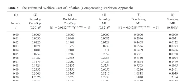
Table 8. The Estimated Welfare Cost of Inflation (Compensating Variation Approach)
(1) (2) (3) (4) (5) (6) (7)
Interest
Semi-log Cur.-Dep.
Double-log Cur.-Dep.
Semi-log M1
Double-log M1
Semi-log MB
Double-log MB
i (0.301)i2 [(120.0182i0.5760)20.736221] (0.821)i2 [(120.0478i0.5546)20.803121] (0.304)i2 [(120.0172i0.5612)20.781921]
0.00 0.0000 0.0000 0.0000 0.0000 0.0000 0.0000
0.01 0.0030 0.0944 0.0082 0.2996 0.0031 0.1015
0.02 0.0120 0.1408 0.0328 0.4408 0.0122 0.1499
0.03 0.0271 0.1779 0.0739 0.5526 0.0273 0.1882
0.04 0.0481 0.2101 0.1314 0.6489 0.0486 0.2213
0.05 0.0752 0.2389 0.2052 0.7351 0.0760 0.2509
0.06 0.1082 0.2655 0.2956 0.8140 0.1094 0.2780
0.07 0.1473 0.2902 0.4023 0.8874 0.1489 0.3032
0.08 0.1924 0.3135 0.5254 0.9563 0.1945 0.3269
0.09 0.2435 0.3356 0.6650 1.0216 0.2461 0.3493
0.10 0.3006 0.3567 0.8210 1.0838 0.3039 0.3707
0.20 1.2026 0.5328 3.2839 1.6010 1.2154 0.5481
0.30 2.7058 0.6740 7.3888 2.0138 2.7347 0.6892
0.40 4.8102 0.7966 13.136 2.3715 4.8616 0.8111
0.50 7.5160 0.9071 20.524 2.6934 7.5963 0.9204
0.60 10.823 1.0087 29.555 2.9896 10.939 1.0207
0.70 14.731 1.1035 40.228 3.2662 14.889 1.1142
0.80 19.241 1.1930 52.542 3.5273 19.447 1.2020
0.90 24.352 1.2780 66.500 3.7755 24.612 1.2854
1.00 30.064 1.3592 82.097 4.0130 30.385 1.3649
Note: This table presents the estimated welfare cost of inflation in both the currency-deposit model and the single-monetary-asset model using Lucas’ compensating variation approach with two different functional forms (semi-log, double-log) and three different monetary aggregates (currency-deposit, M1, and monetary base). Entries are multiplied by 100 and can thus be interpreted as percentages.
T.
G.
equation (8), which yields the double-log asset demand functions shown in equations (9a) and (9b). With equations (9a) and (9b), the equilibrium conditions (21a) and (21b) imply:
m#~i!5
S
mt ctD
5
S
g2 g1D
it
2u (26a)
d#~mi!5
S
dt ctD
5
S
g3 g1D
~mtit!
2u (26b)
The welfare cost is defined as the solution w(i) to u[11w(i), m#(i), d# (mi)]5u(1`,`).
With the CES utility assumed in equation (8), the right side is finite providedu,1, which is to say, provided the elasticity of substitution between goods consumption and real currency and the elasticity of substitution between goods consumption and real deposits are less than one. Using equations (26a), (26b), and the utility function in equation (8), we find that:12
w~i!5
F
12S
g2 g1D
it
12u2
S
g3g1
D
mt12u it
12u
G
u/~u21!21. (27)
The exact welfare cost of inflation w(i) given in equation (27) is calibrated by employing the estimated parameter values. For the double-log form with the currency– deposit specification,13,u5 0.4240 (orb150.4240 in footnote 13), g2/g150.0134 (or e
b05
e24.3109in footnote 13) andg3/g150.0149 (or e
b25e24.2063in footnote 13). The implied
welfare cost function evaluated at the mean of the reserve ratiommean50.1373 is thus: 14
w~i!5~120.0182it0.5760!20.736221. (28)
The third column of Table 8 presents some values of this function, which yields a welfare cost of a 10 percent nominal interest rate at about 0.36 percent of GDP. Reduction to a zero inflation rate (or a 3 percent nominal rate) reduces the cost to about 0.18 percent, for a gain of about 0.18 percent of GDP. Therefore, compared to the semi-log function, the
12The CES utility function presented in equation (8) implies
u~1,`,`!5@~g1
1/u!u/~u21!#12s1
121 s
u@11w~i!,m#~i!,d#~mi!#5$@g1 1/u
~11w~i!!~u21!/u1g 2 1/u
m#~i!~u21!/u1g 3 1/u
d#~mi!~u21!/u#u/~u21!
%121
s
121 s
wherem#~i! 5
S
g2 g1D
i2uandd#~mi! 5
S
g3 g1D
~mi!2u. Solving u[11w(i), m
#(i), d#(mi)]5u(1,`,`) for w(i) yields the exact welfare cost of inflation presented in equation (27).
13In the restricted case where we assume the demand for currency and deposits have the same elasticity, the
long-run regression coefficients, obtained from the estimated asset demand equations with the double-log form:
log (m/y)t5b02b1log itand log (d/y)t5b22b1log (mtit), are found to beb05 24.3109 (29.1084),b15
0.4240 (2.6511) andb25 24.2063 (25.0218) with t ratios in parentheses.
14Lucas (1994) uses an estimate of the semi-elasticity (h57) of demand for M1 in the
single-monetary-asset model obtained from 1900 to 1985 annual U.S. time series to obtain the interest elasticity (u5hi), which
turn out be about 0.5. Then he finds the welfare cost estimate as: w(i)5(120.045it
0.5)2121>0.045i
t
0.5, which
double-log function yields a substantial welfare gain (0.18 percent of GDP) of moving from zero inflation to the steady deflation of around 3 percent.
To determine the degree of overestimation due to the identification of money with M1, the same procedure is followed to find w(i) for M1, usingu50.4454 (orb150.4454 in Table 5) andg2/g150.0478 (or e
b05e23.0405in Table 5). The exact welfare cost w(i)
for M1 is therefore:15
w~i!5~120.0478it
0.5546!20.803121. (29)
The fifth column of Table 8 displays some values of this function, which gives a substantial welfare cost of 1.08 percent of GDP at the 10 percent nominal interest rate. Reduction to a zero inflation rate reduces the cost to about 0.55 percent, for a considerable gain of about 0.53 percent of GDP.
We now present the exact welfare cost of inflation w(i) for the monetary base using the estimated parameter valuesu50.4388 (orb150.4388 in Table 5) andg2/g150.0172 (or eb05 e24.0635in Table 5). The implied welfare cost function is thus:
w~i!5~120.0172it0.5612!20.781921. (30)
The last column of Table 8 demonstrates some values of this function. At the 10 percent nominal interest rate the welfare cost is about 0.37 percent of GDP. Reduction to a zero inflation rate reduces the cost to about 0.19 percent, for a gain of about 0.18 percent of GDP. Therefore, compared to the semi-log function, the double-log function with the monetary base implies substantial welfare gains (0.19 percent of GDP) associated with moving from zero inflation to the steady deflation of around 3 percent.
As an alternative to the compensating variation approach of Lucas discussed above, we will now introduce Bailey’s consumer surplus approach to estimate the welfare cost of inflation in the currency– deposit model using the semi-log and the double-log forms of asset demand functions. Deadweight social costs of raising revenue via seigniorage collection can be interpreted as the lost areas under currency and deposit demand curves owing to inflation’s effect on their respective opportunity costs. This is the traditional “shoe-leather” cost developed by Bailey (1956). With the general form of currency and deposit demand functions, the welfare cost (WC) is measured as the deadweight loss from positive i in reducing currency demand,
E
0 i
f~x!dx2if~i!, (31a)
plus the deadweight loss from positive mi in reducing deposit demand,
15In the single-monetary-asset model, the exact welfare cost of inflation w(i) is defined as the solution to:
u[11w(i), m#(i)]5u(1,`). With the following CES utility function,
u~ct,mt! 5 $@g11/uct
~u21!/u1g 2 1/um
t
~u21!/u#u/~u21!%12s1
121 s
, we find that:w~i! 5
F
1 2S
g2 g1D
it
12u
G
u/~u21!E
0 mi
g~x!dx2mig~mi!. (31b)
Hence, with the semi-logarithmic form of currency and deposit demand, the welfare cost of inflation (as a fraction of GDP) is defined as follows,16
WCBaileysemi-log5
E
0 i
ea02a1xdx2ea02a1ii1
E
0 mi
eb02b1xdx2eb02b1mi~mi! (32a)
WCBailey semi-log5e
a0
a1
~12e2a1i~11a
1i!!1
eb0
b1
~12e2b1mi~11b
1mi!!, (32b)
and with the double-log form,
WCBaileysemi-log5
E
0 i
ea0x2a1dx2ea0i12a11
E
0 mi
eb0x2b1dx2eb0~mi!12b1 (33a)
16Most of the estimates displayed in Tables 3 and 4 have the Box–Cox parameterl,0, rather than 0, l,1. Because one of this paper’s main messages is that accurate estimation of the welfare loss must be based on the correct specification of money demand, the reader may think that the welfare cost function obtained from the nonlinear form of money demand should be introduced and discussed. However, there is no closed form or numerical solution to the welfare cost of inflation when the nonlinear, Box–Cox form of money demand is employed. To see this, consider the following welfare cost function with the nonlinear specification we are using:
S
WC yD
nonlinear 5
E
0
i
ea02a1
S
xl121
l1
D
dx2ea02a1S
il121
l1
D
i1E
0 mi
eb02b1
S
xl221
l2
D
dx2eb02b1S
~mi!l221 l2
D
~mi!,which does not have an analytical solution. For a given value of i andm, this expression does not yield a numerical solution even the estimated parameters (a’s,b’s,l’s) are plugged in. To see at least approximately how larger or smaller the welfare cost estimates will be when the nonlinear form is used, we plot the double-log and nonlinear demand functions. The appropriate area under the nonlinear demand curve turns out to be almost the same as the one under the double-log function.
In addition, as described in Section IV, finding a welfare cost formula with the compensating variation approach requires a specific form for both the utility and the asset demand functions. Because there is no analytical solution to the utility function,
u~mt,dt,ct!5
E
0
m/c
e
1
1n
S
a0l1a12l1n~x!
a1
l
2
dx1E
0
d/c
e
1
1n
S
a0l1a12l1n~y!
a1
l
2
d y1v~c!,WCBailey double-log
5
S
a112a1
D
ea0i12a11
S
b112b1
D
eb0~mi!12b1. (33b)
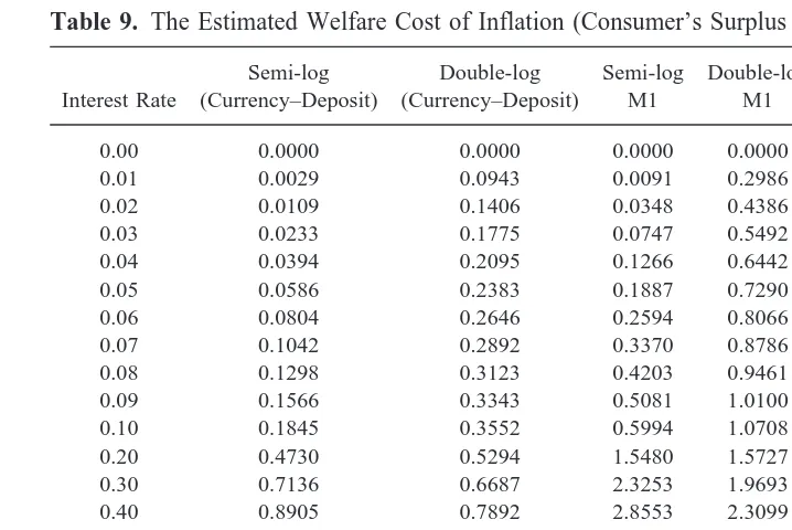
Our first important observation is that there is almost no difference between the magni-tudes of the welfare cost of inflation estimated in Bailey’s partial equilibrium and Lucas’s general equilibrium frameworks.17In other words, we obtain the same result that for each monetary aggregate (currency– deposit, monetary base, M1), the double-log function implies sizable benefits in moving from zero inflation to the steady deflation of around 3 percent that would attain the Friedman optimum, while under semi-log demand these benefits are trivial. The reader may wish to consult Table 9 to see the sensitivity of the estimated welfare cost of inflation to the specification of money demand and to the
17Driffill et al. (1990) show that the two approaches—consumer’s surplus and compensating variation—are
equivalent if inflation is assumed to leave real wealth and real interest rate unaffected. This assumption can be taken to apply only to short-run costs of inflation. But, in the long-run, inflation may affect both real wealth and real rate of interest. In that case, the consumer’s surplus argument is not an exact measure of welfare change. Driffill et al. (1990) mention that there are three reasons why inflation might be expected to have long-run effects on the real rate of interest and real income or wealth. First, as Tobin (1955, 1965) noted, higher inflation in reducing the demand for real money balances may cause a switch in the portfolio of assets held in the economy; in particular, lower real money balances may cause an increase in holdings of physical capital, and this would raise output per capita and reduce the real interest rate. This is the “Tobin” effect. Second, as Feldstein (1976) noted, in addition to these portfolio effects there may be savings effects if the saving rate depends on the real rate of interest as would be suggested by life-cycle models of savings. Finally, depending on assumptions about the structure of taxation, higher inflation rates will have implications for the government budget constraint and these offsetting fiscal policies may have further effects.
Table 9. The Estimated Welfare Cost of Inflation (Consumer’s Surplus Approach)
Interest Rate
Semi-log (Currency–Deposit)
Double-log (Currency–Deposit)
Semi-log M1
Double-log M1
Semi-log MB
Double-log MB
0.00 0.0000 0.0000 0.0000 0.0000 0.0000 0.0000
0.01 0.0029 0.0943 0.0091 0.2986 0.0031 0.1014
0.02 0.0109 0.1406 0.0348 0.4386 0.0119 0.1496
0.03 0.0233 0.1775 0.0747 0.5492 0.0256 0.1878
0.04 0.0394 0.2095 0.1266 0.6442 0.0434 0.2207
0.05 0.0586 0.2383 0.1887 0.7290 0.0648 0.2502
0.06 0.0804 0.2646 0.2594 0.8066 0.0892 0.2771
0.07 0.1042 0.2892 0.3370 0.8786 0.1160 0.3022
0.08 0.1298 0.3123 0.4203 0.9461 0.1449 0.3257
0.09 0.1566 0.3343 0.5081 1.0100 0.1753 0.3479
0.10 0.1845 0.3552 0.5994 1.0708 0.2071 0.3691
0.20 0.4730 0.5294 1.5480 1.5727 0.5406 0.5447
0.30 0.7136 0.6687 2.3253 1.9693 0.8193 0.6838
0.40 0.8905 0.7892 2.8553 2.3099 1.0132 0.8037
0.50 1.0200 0.8975 3.1861 2.6142 1.1366 0.9109
0.60 1.1203 0.9968 3.3821 2.8924 1.2112 1.0090
0.70 1.2040 1.0894 3.4943 3.1506 1.2548 1.1002
0.80 1.2787 1.1764 3.5570 3.3927 1.2796 1.1858
0.90 1.3485 1.2590 3.5914 3.6218 1.2935 1.2668
1.00 1.4154 1.3378 3.6100 3.8397 1.3012 1.3440
definition of money with Bailey’s approach. Second, the welfare cost measures in the currency– deposit model turn out to be almost the same as those in the single-monetary-asset model when the monetary base is identified as the relevant definition of money. Defining M1 without modeling the distinctive roles of currency and deposits as the appropriate money overestimates the true welfare cost of inflation in both the consumer’s surplus and compensating variation approaches.
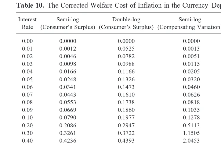
The above welfare cost analysis in the currency– deposit model does not account for the significant magnitude of U.S. currency held overseas, which shifts a sizable part of the welfare cost abroad. Because a considerable fraction of U.S. currency is held abroad, the welfare cost estimates based on currency in the paper overstates the actual cost of inflation. How much U.S. currency is abroad is important for welfare cost estimates although currency movements are extremely difficult to measure, and estimates of the foreign component of currency stocks and flows are subject to a great deal of speculation and uncertainty. Porter and Judson (1996) have examined ten methods for estimating the amount of currency held abroad.18In their summary of all estimation methods, they derive an extreme range of 49 percent to 71 percent for the foreign share of currency and then they say neither endpoint is likely to be correct, whereas a value near the middle, which is 60 percent, is much more likely to be so. Thus, I use the midpoint (60 percent) as a rough measure of the percentage of U.S. currency held abroad and re-estimate the welfare loss in the currency– deposit model. The corrected welfare cost estimates are presented in Table 10.
V. Conclusions
This paper emphasizes that it is crucial to identify the proper specification of money demand as well as the appropriate monetary aggregate to find the exact welfare cost of inflation. The empirical results obtained from the nonlinear form of money demand with Box–Cox restriction indicate that the double-log function with constant elasticity of less than one is a more accurate characterization of the actual data than the semi-logarithmic form commonly used.
This study quantifies the welfare loss of deviating from a zero inflation policy and determines how much welfare the U.S. gains in moving from zero inflation to the Friedman optimal deflation rate. The welfare cost measures obtained from Bailey’s consumer’s surplus and Lucas’s compensating variation approaches turn out to be almost the same. Compared to the constant semi-elasticity Cagan-type demand for money, the constant elasticity double-log function yields substantial costs of deviating from both a zero inflation policy and an optimal deflation policy in both the currency– deposit model and the single-asset monetary model.
Using the double-log form of currency and deposit demand functions, we find the welfare cost of a sustained 4 percent inflation is around 0.29 percent of GDP and the welfare gain in moving from a 4 percent to a zero inflation rate is computed as around 0.11 percent of GDP. In the single-monetary-asset model, these welfare cost estimates are not affected when the monetary base is used as the relevant definition of money. However, when M1 is identified as the appropriate monetary aggregate the aforementioned measures
18The currency–deposit model developed in Section II does not account for U.S. currency held overseas but
calculated with the currency– deposit specification or with the monetary base are inflated to 0.89 percent of GDP (welfare cost of a 4 percent inflation) and 0.34 percent of GDP
(welfare gain in moving from p 5 4 percent to p 5 0). With the currency– deposit
specification or with the monetary base, the additional gain in moving from zero inflation to zero nominal rate that would attain the Friedman optimum is found to be around 0.18 percent of GDP whereas with M1 it is overestimated as 0.55 percent of GDP.
The welfare cost measures discussed above are calculated by using income as the quantity variable. In addition to income, we also use consumption as the scale variable in estimating the welfare loss for the U.S. economy. The welfare cost estimates as a percentage of consumption turn out to be proportionately higher (without affecting our conclusions) because the ratio of consumption to GDP is around two-thirds in the United States.
I owe a great debt to Alvin L. Marty and Thom B. Thurston for their helpful suggestions at every stage of the work. I also benefited from discussions with Salih N. Neftci on certain theoretical and empirical points. I would like to thank Kenneth Kopecky, David VanHoose, and two anonymous reviewers of this journal for their helpful comments and suggestions on earlier versions of the paper. Many thanks go also to seminar participants at the 24th Meeting of the Eastern Economic Association.
References
Baba, Y., Hendry, D. F., and Starr, R. M. 1992. The demand for M1 in the U.S.A., 1960–1988.
Review of Economic Studies 59:25–61.
Table 10. The Corrected Welfare Cost of Inflation in the Currency–Deposit Model
Interest Rate
Semi-log (Consumer’s Surplus)
Double-log (Consumer’s Surplus)
Semi-log (Compensating Variation)
Double-log (Compensating Variation)
0.00 0.0000 0.0000 0.0000 0.0000
0.01 0.0012 0.0525 0.0013 0.0526
0.02 0.0046 0.0782 0.0051 0.0784
0.03 0.0098 0.0988 0.0115 0.0991
0.04 0.0166 0.1166 0.0205 0.1170
0.05 0.0248 0.1326 0.0320 0.1330
0.06 0.0341 0.1473 0.0460 0.1478
0.07 0.0443 0.1610 0.0626 0.1616
0.08 0.0553 0.1738 0.0818 0.1746
0.09 0.0669 0.1860 0.1035 0.1869
0.10 0.0790 0.1977 0.1278 0.1986
0.20 0.2086 0.2947 0.5113 0.2967
0.30 0.3261 0.3722 1.1505 0.3753
0.40 0.4236 0.4393 2.0453 0.4435
0.50 0.5063 0.4996 3.1958 0.5051
0.60 0.5804 0.5549 4.6019 0.5616
0.70 0.6499 0.6064 6.2637 0.6144
0.80 0.7171 0.6549 8.1812 0.6643
0.90 0.7831 0.7009 10.354 0.7116
1.00 0.8480 0.7447 12.783 0.7568
Bailey, M. J. 1956. The welfare cost of inflationary finance. Journal of Political Economy 64:93–110.
Banerjee A., Dolado, J., Galbraith, J. W., and Hendry, D. F. 1993. Co-integration, Error-Correction,
and the Econometric Analysis of Non-Stationary Data. Oxford: Oxford University Press.
Calvo, G. A., and Fernandez, R. B. 1983. Competitive banks and the inflation tax. Economics
Letters 12:313–317.
Cagan, P., 1956. The monetary dynamics of hyperinflation. In Studies in the Quantity Theory of
Money, (M. Friedman, ed.). Chicago: University of Chicago Press, pp. 24–117.
Clower, R.W., 1967. A reconsideration of the microfoundations of monetary theory. Western
Economic Journal 6:1–8.
Daniels, J. P., and VanHoose, D. D. 1996. Reserve requirements, currency substitution, and seigniorage in the transition to European Monetary Union. Open Economies Review 7:257–273. Dickey, D. and Fuller, W. A. 1979. Distribution of the estimates for autoregressive time series with
a unit root. Journal of the American Statistical Association 74:427–431.
Dotsey, M. and Ireland, P. 1996. The welfare cost of inflation in general equilibrium. Journal of
Monetary Economics 37:29–47.
Driffill, J., Mizon, G. E., and Ulph, A. 1990. Costs of inflation. In Handbook of Monetary
Economics, Vol. 2, (B. M. Friedman and F. H. Hahn, eds.). New York: North Holland.
Eckstein, Z., and Leiderman, L. 1992. Seigniorage and the welfare cost of inflation. Journal of
Monetary Economics 29:389–410.
Engle, R.E. and Granger, C. W. J. 1987. Cointegration and error-correction: Representation, estimation, and testing. Econometrica 55:251–276.
Feldstein, M. S. 1976. Inflation, income taxes, and the rate of interest—A theoretical analysis.
American Economic Review 66:809–820.
Fischer, S. 1981. Towards an understanding of the costs of inflation: II. Carnegie–Rochester
Conference Series on Public Policy 15:5–41.
Friedman, M. 1969. The optimum quantity of money. In The Optimum Quantity of Money and Other
Essays. Chicago: Aldine.
Hendry, D. F. 1980. Predictive failure and econometric modeling in macroeconomics: The trans-actions demand for money. In Economic Modeling. London: Heinemann Education Books. Hwang, H. 1985. Test of the adjustment process and linear homogeneity in a stock adjustment model
of money demand. The Review of Economics and Statistics LXVII:689–692.
Lucas, R. E., Jr. 1981. Discussion of: Stanley Fischer, ‘Towards an understanding of the costs of inflation: II.’ Carnegie–Rochester Conference Series on Public Policy 15:43–52.
Lucas, R. E., Jr. 1994. On the welfare cost of inflation. Working paper 394, (Stanford University, Center for Economic Policy Research).
Lucas, R. E., Jr., and Stokey, N. L. 1983. Optimal fiscal and monetary policy in an economy without capital. Journal of Monetary Economics 12:55–93.
Marty, A. L. 1976. A note on the welfare cost of money creation. Journal of Monetary Economics 2:121–124.
Marty, A. L., and Chaloupka, F. J. 1988. Optimal inflation rates: A generalization. Journal of
Money, Credit, and Banking 20:141–144.
Marty, A. L. 1994. The inflation tax and the marginal welfare cost in a world of currency and deposits. Federal Reserve Bank of St Louis July/August:25–29.
McCallum, B.T. 1983. The role of overlapping-generations models in monetary economics.
Carn-egie–Rochester Conference Series on Public Policy 18:9–44.
McCallum, B.T. and Goodfriend, M.S. 1988. Demand for money: Theoretical studies. Federal
Reserve Bank of Richmond Economic Review 74:16–24.
Porter, R. D., and Judson, R. A. 1996. The location of U.S. currency: How much is abroad? Federal
Rose, A. 1985. An alternative approach to the American demand for money. Journal of Money,
Credit, and Banking 17:439–455.
Sidrauski, M. 1967. Rational choice and patterns of growth in a monetary economy. American
Economic Review 57:534–544.