www.elsevier.com / locate / econbase
On the mean-reverting properties of target zone exchange rates:
a cautionary note
a ,
*
bMark P. Taylor
, Matteo Iannizzotto
a
Warwick Business School, University of Warwick, Coventry CV4 7AL, UK b
Department of Economics and Finance, University of Durham, 23 –26 Old Elvet, Durham DH1 3HY, UK Received 23 March 2000; accepted 15 July 2000
Abstract
We estimate a franc–mark target zone model and find a very limited ‘honeymoon effect’. Monte Carlo experiments calibrated with the estimates caution against the use of standard linear tests for non-mean reversion as indirect tests of the target zone model. 2001 Published by Elsevier Science B.V.
Keywords: Exchange rates; Target zones; Mean-reversion
JEL classification: F31; F33
1. Introduction
The purpose of this note is twofold. First, we estimate a target zone exchange rate model of the kind originally suggested by Krugman (1991) and further developed and extended by, inter alios, Froot and Obstfeld (1991) and Flood and Garber (1992); (see Bertola and Caballero, 1992; Svensson, 1992 and Taylor, 1995 for surveys), using daily French franc–German mark data and employing the method of simulated moments estimator. Our parameter estimates, while statistically significant and plausible in magnitude and in line with the literature on estimated elasticities of money demand, imply that the degree of non-linearity in target zone exchange rates – the so-called ‘honeymoon effect’ – is very much smaller than has hitherto been implicitly assumed to be the case. Second, through a battery of Monte Carlo experiments calibrated on our estimated model, we demonstrate that standard tests for non-mean reversion of exchange rates such as Dickey-Fuller or variance ratio tests, may have very little power even when the data is generated by a fully credible target zone arrangement. This cautions
*Corresponding author. Tel.: 144-2476-572-832; fax: 144-2476-573-013.
E-mail addresses: [email protected] (M.P. Taylor), [email protected] (M. Iannizzotto).
against the use of such tests as indirect tests of the model, contrary to the suggestion of a number of authors.
2. Data
We use daily data for the French franc–German mark over the longest period of stability available (i.e. without realignments to satisfy the assumption of full credibility of the band, Krugman, 1991), from 12th January 1987 to 9th April 1992, obtained from the Bank for International Settlements data base. To facilitate interpretation of our parameter estimates, the data were expressed as percentage
1
deviations from the central parity .
3. The target zone model
Define the nominal exchange rate, S(t), to be a function of a fundamental term, x(t), and of its own rate of instantaneous expected depreciation:
E dS tf s dg
]]]
S ts d5x ts d1a (1)
dt
The parameter a represents the interest rate semi elasticity of money demand from the original equations of the monetary model that underlies Eq. (1) (see e.g. Taylor, 1995). The fundamental itself is assumed to behave as a Brownian motion:
dx5hdt1sdw (2)
whereh represents the drift parameter, s the standard deviation and dw the increment of a standard ˆ
Wiener process. Using Ito’s lemma to solve for the instantaneous rate of depreciation results in a second order differential equation the solution to which is of the form:
S5x1ah1A exp1 sl1xd1A exp2 sl2xd
where A and A are arbitrary constants to be determined by the smooth pasting conditions, which1 2
l u
require the first derivative of S to be zero at the boundaries. The terms x and x are, respectively, the
1
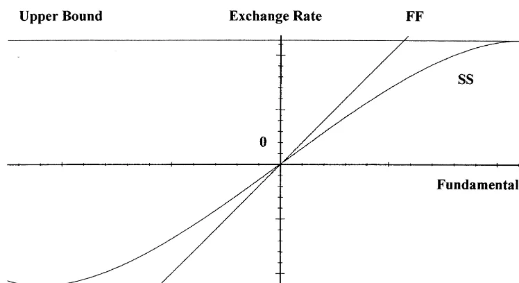
Fig. 1. Target zone model of exchange rates.
lower and upper bounds of the fundamental andl1,2 are the two roots of the characteristic equation of the second-order differential equation and, for clarity of exposition, the argument t has been dropped from S and x.
Fig. 1 depicts the relationship between the exchange rate and the fundamental in the target zone model, SS (Eq. (3)), compared with the relationship which would obtain under a free float, FF (Eq. (1) with the expected change in the exchange rate set to zero), and is drawn with a reasonable amount of curvature in the SS line (compare the similar figures in, for example, Krugman, 1991; Svensson, 1992 and Taylor, 1995). The curvature of the SS line in fact represents the ‘honeymoon effect’ whereby the credibility of intervention at the bands is built into agents’ expectations and pushes the SS line below FF above the central parity and above FF below the central parity. This means that during the ‘honeymoon’ of credibility, the authorities are allowed a greater degree of flexibility in the fundamentals for any given range of fluctuation of the exchange rate than would be the case under a free float. In discussions of credible target zone arrangements in the literature, the honeymoon effect appears to have been viewed as one of the key attractive features of such arrangements.
4. The method of simulated moments
Direct econometric estimation of the basic target zone model has previously been attempted with the method of simulated moments (MSM), albeit with limited success, for both ERM currencies
¨
(Smith and Spencer, 1992; De Jong, 1994) and the Nordic target zone (Lindberg and Soderlind, 1994). The MSM is convenient in that it provides a way of circumventing the problem of a vaguely defined, possibly very complicated fundamentals term. The MSM estimator (Lee and Ingram, 1991; Duffie and Singleton, 1993) is based on the iterated generation of artificial data by a computer
3
statistical moments of the artificial data, averaged across the large number of replications, are computed and compared with the statistical moments of the actual data. A loss function, which weighs, in an appropriate metric, the deviations between the simulated and the actual moments, is minimised recursively by changing the parameter values until the algorithm converges and further reductions in the loss function become negligible. The parameter values thus obtained are the MSM estimates. Formally, define
as the sample moments of, respectively, the observed data (k , zz 51, . . . ,Z ) for Z observations; and the simulated data, conditional on a vector of parameters b, ( y (j b), j51, . . . ,N ) for N simulated observations. In the present instance, the observed data are daily ERM exchange rates, the parameter vector is composed of the three parameters of the Krugman model b5(a h s)9, and the simulated data are generated values, according to Eq. (3), given a specific parameter vector for each simulation. Lee and Ingram (1991) show that under weak regularity conditions and given a symmetric weighting matrix W , the Simulated Moments Estimator is found by minimising the following lossZ
function with respect to the parameter vector b:
L5hH kZs d2H yNf s dgb j9W H kZh Zs d2H yNf s dgb j. (5)
*
Hansen (1982) shows that W , defined as follows, is an optimal choice for the weighting matrix in theZ sense that it yields the smallest asymptotic covariance matrix for the estimator:
21
Given W , the MSM estimator converges in distribution to the normal:Z
21 21
population moments of the observed process, and n5N /Z is the ratio of the length of the simulated
3
series over the length of the observed series.
In order to test whether the moment restrictions imposed on the model are true, we exploit the
2
For the estimation of the covariance matrix of the estimated parameters to be implemented, a consistent estimate ofV
can be found following the method of Newey and West (1987). 3
result proved by Hansen (1982) that, under the null hypothesis of no errors in specification, the minimised value of the criterion function converges asymptotically to a chi-square distribution. The number of degrees of freedom of this specification test is equal the difference between the number of moment conditions (m) and the number of parameters being estimated (k):
D 2
ˆ
*
ˆZ H k
h
Zs d2H yNf s dgj
bZN 9WZh
H kZs d2H yNf s dgj
bZN →x sm2kd (8)5. Estimation results
Five moments conditions are used to estimate three parameters, namely: a, the interest rate semi-elasticity;h, the drift parameter, and s, the standard deviation of the fundamental.
The estimates are presented in Table 1. They are all significant at conventional levels and the Hansen test of over-identifying restrictions does not reject the moments restrictions imposed for the
2
estimation: its value is 0.085231 and its marginal significance level (x with two degrees of freedom under the null hypothesis) is 0.96.
Since we are unable to reject the target zone model on the basis of this specification test, the question now arises of what our estimates imply in terms of Eq. (3). By substituting these values in place of the corresponding parameters we obtain:
2.6594 3.2451 7.5063
]]] ]]] ]]]
SFF5x1 4 2 26 exp(23.964x)1 26 exp(224.118x) (9)
10 10 10
The complementary function, represented by the last two terms on the right-hand-side of Eq. (9), virtually vanishes because of the magnitude of the two constants of integration (both scaled by a
226
factor 10 ). The determination of S therefore, within a certain range, is to a large extent solely dependent on the value of x, the stochastic fundamental. As a result this function is for all practical purposes a 458 degree line in S –x space which represents also the free-float solution of the model when no intervention is expected from the monetary authorities and the exchange rate simply equals the fundamental. The non-linearity postulated by the theoretical model is indeed present but it only applies in the very close neighbourhood of the tangency point at the edges of the band. Fig. 2 provides
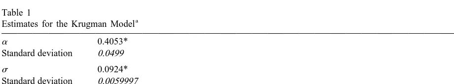
Table 1
a Estimates for the Krugman Model
a 0.4053*
Standard deviation 0.0499
s 0.0924*
Standard deviation 0.0059997
h 0.00065616*
Standard deviation 0.00004974 a
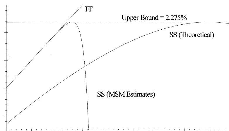
Fig. 2. Close-up of the point of tangency with the upper bound.
a graphical representation of this feature, where a close-up of the point of tangency with the upper
4 5
bound is depicted for both Eq. (9) and the SS curve depicted in Fig. 1. This is an interesting result as it implies that, although the target zone model does find support in the data, the theoretical ‘honeymoon effect’ can be so small in magnitude as to have hardly any practical effect. It is therefore possible that the theoretical target zone literature may have overestimated the magnitude of the ‘honeymoon effect’ so that the consistent failure to detect empirically a strongly non-linear relationship between the exchange rate and the fundamentals in a target zone arrangement may have led to an unwarranted dismissal of the basic target zone model. Admittedly, however, this point is crucially dependent on the plausibility of the parameter estimates.
We believe our estimates to be plausible. In the case ofa, the parameter on whose value most of the empirical literature has concentrated, Flood et al. (FRM) (1991), for instance, suggest that a value
6
of a50.1 is ‘ . . . a reasonable value . . . ’. They, however, measure their interest rates in decimals
and on an annualised basis. Since we use daily exchange rate data expressed in percentage deviations from the central parity, our estimated semi-elasticity is in different units from that of FRM. To convert the FRM value ofa to the same units as our estimate, we need to divide by 100 (to allow for the fact
4
The upper bound is at 2.275% and the lower one at 2.225% from the central parity. The ERM was in fact slightly asymmetric in order for any two central banks to have the same intervention points, at the margin, whilst the central parity was defined, for one of them, as the inverse of what was for the other one. A mechanical application of a symmetric band would have resulted in a linear transformation of a non linear relationship, and therefore in discrepancies at the edges of the band. This is a form of the Siegel paradox.
5
In the present instance the ‘theoretical SS’ is obtained by setting a 510,h 50 and s 51.0. 6
FRM used interest data expressed in decimals) and multiply by 365 (to allow for the fact that FRM used interest rates expressed on an annualised basis). Thus, FRM’s suggested reasonable value of a
becomes (0.1 / 100)336550.365. This is of the same order of magnitude as our estimated value of 0.4053. Moreover, since our estimated value is greater than the value suggested as reasonable by FRM, this will if anything tend to increase the honeymoon effect.
Our estimate ofa can also be compared with previous research on money demand equations. To do this, we need to divide our estimate (0.4053) by 365 (days) in order to put it on an annualised basis. Also, to turn it from a semi-elasticity into an elasticity, we need to multiply it by an interest rate of, say, 10%. Therefore the implied interest rate elasticity at an annualised interest rate of 10% turns out to be (0.4053 / 365)31050.011. Interestingly, this is very close to the figure of 0.015 quoted by Bilson (1978) as the most plausible prior for the interest rate elasticity of money demand at a 10%
7
annual interest rate, based on a reading of the empirical literature on money demand.
To obtain the sort of curves displayed in most theoretical papers, one would have to increase the
8
interest rate semi-elasticity to totally implausible values like 10 or 20.
6. Monte Carlo experiments
If the honeymoon effect is as slight as our estimation results suggest, then except in the close neighbourhood of the target zone bands, the exchange rate will behave largely as it does under a free float (graphically, the SS and FF lines coincide in Fig. 2 for nearly all of the allowed range of fluctuation). Since under a free float the exchange rate will simply inherit the Brownian motion in the fundamentals, it therefore seems likely that tests for mean reversion of the exchange rate – even when it is determined within a fully credible target zone – may greatly lack power to reject the false null hypothesis of a unit root.
To demonstrate this point, we artificially simulated data constructed using Eqs. 2 and 3, calibrated using our estimated parameters and using a random number simulator to generate the stochastic
9
innovations in the fundamentals. The artificial series we constructed was in each case of 2015 days in length. We then discarded the first 100 observations, leaving a data series matching in length that of our estimation period. We then discarded observations corresponding to the pattern of missing values resulting from holidays and weekends in our actual data set. We then performed Dickey-Fuller and an augmented Dickey-Fuller tests for non-mean reversion on the constructed data, with an algorithm which allows at first a generous lag length (20) and then progressively reduces the lag length based on the significance of the estimated parameters, to achieve an optimal specification of the test. Both tests were performed including and excluding a time trend and in both cases we used the 5% critical values calculated from the response surface estimates of MacKinnon (1991). This process was repeated 5000
7
Our estimate for the fundamental standard deviation implies an annual standard deviation of 0.09243œ(365), or about 2%, which does not seem to be unreasonable.
8
Iannizzotto and Taylor (1999) provide a graphical analysis of this issue. 9
times and we then calculated the percentage of times we were able to reject the null hypothesis of a unit root.
At each replication, we also applied variance ratio tests for the null hypothesis of random walk behaviour of the exchange rate. The variance ratio tests considered were the two specifications (which we term c1 and c2) presented in Campbell et al. (1997). These tests exploit the fact that, under the null hypothesis of a random walk for a given series S(t), the variance of discrete increments must be a linear function of the time interval. For example, if we normalise on a specific time interval – say 1 day – then DS(t);S(t)2S(t21) is the daily increment. Then, if S(t) follows a random walk, the variance of [DS(t)1 DS(t21)1 . . . 1 DS(t2q)] must be q times the variance ofDS(t). Put another
way, the ratio of the two quantities Var[DS(t)] and (1 /q)Var[DS(t)1 DS(t21)1 . . . 1 DS(t2q)]
must be unity. Variance ratio tests are based on the distribution of estimators of this ratio. Consider the
2 2
¯ ¯
following two unbiased and consistent estimators of these variances, sa and sc, based on T11 observations indexed from 0 to T :
T 2
Campbell et al. (1997) use Eqs. (10) and (11) to define the following two variance ratio test t-statistics, c1 and c2, given the variance ratio VR( q):
2
The variance ratioc2 is robust to the presence of heteroskedasticity in the errors of the series and it is therefore of much greater importance in applications to financial series which generally exhibit a significant degree of heteroskedasticity. The term Q( q) is defined as:
Table 2
We considered the tests with three values of the lag length ( q) used for computing the autocorrelation terms: namely q58, 16 and 24. For the variance ratio statistics, corrections of the critical values at the 5% significance level were obtained by separate Monte Carlo simulation (with data generated under the null hypothesis) to obviate the bias in the distribution of the tests. In the case of c2, we estimated a second-order autoregressive conditionally heteroskedastic – i.e. ARCH(2) – model of changes in the exchange rate series, in order to have a pattern of heteroskedasticity that we
10
could use to generate the simulated data under the null hypothesis (Engle, 1982). This was of the form: Critical values at 5% significance level
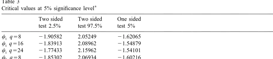
Two sided Two sided One sided test 2.5% test 97.5% test 5%
c1 q58 21.90582 2.05249 21.62065
The variance ratio statistics should be close to zero if the series is a random walk. Values of the statistic that are markedly negative provide evidence of stationarity, while strongly positive ones mean explosive behaviour or mean aversion. The tests can therefore be applied in two ways: a one tailed test which looks for mean reverting behaviour only, and a two tailed test where both mean reversion and aversion are considered as rejections of the null hypothesis of random behaviour. We report the critical values at the 5% significance level for both interpretations.
10
where I(t21) denotes information at time t21. The maximum likelihood estimates of the coefficients of the ARCH model are reported in Table 2; they are all strongly significant at conventional significance levels.
We report in Table 3 the 5% critical values for the two variance ratio test statistics, derived from 5,000 Monte Carlo replications under the null hypothesis that S(t) follows a random walk with normally distributed homoskedastic errors (with a variance equal to the sample variance of DS(t)) in
the case of c1, and under the null hypothesis that S(t) follows a random walk with an ARCH(2) disturbance (with the parameters taken from Table 2) in the case ofc2. These critical values were then used to construct power functions for the c1 and c2 by counting the frequency of rejection in 5,000 replications of data artificially generated from our estimates of the target zone model, as with the Dickey-Fuller and augmented Dickey-Fuller tests.
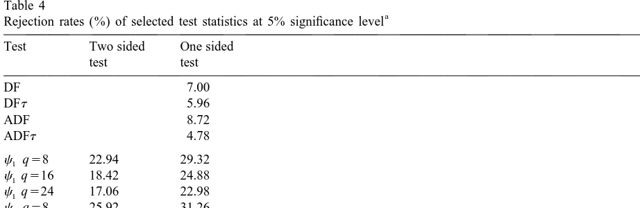
The Monte Carlo results for the power of the Dickey-Fuller and variance ratio unit root tests against the alternative of a fully credible target zone model, calibrated using our estimates from Table 1, are presented in Table 4. The rejection rates are to be interpreted as the probability of correctly rejecting the null hypothesis of a unit root when the target zone model actually holds. For the Dickey-Fuller and augmented Dickey-Fuller tests, the rejection rates are very small indeed, ranging from just under 5% (the chosen significance level) to a little under 9%. The variance ratio tests perform slightly better but are still somewhat lacking in power: the rejection frequencies now range from a minimum of 17.06% to a maximum of 31.26%.
Since, of course, we only have one historical data set, this does not mean that we should expect to reject the unit root hypothesis on between, roughly, 5–30% of occasions – depending on the specific unit root test employed. Rather, the interpretation is that, if our data set were actually generated by a credible target zone model of the kind we have estimated, there is a roughly 70–95% chance that we should never be able to reject the null hypothesis using standard unit root tests, even though it is false.
Table 4
a Rejection rates (%) of selected test statistics at 5% significance level Test Two sided One sided
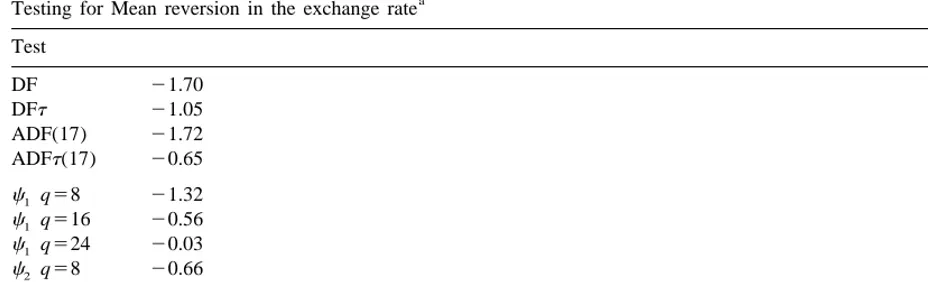
Table 5
a Testing for Mean reversion in the exchange rate Test
DF5Dickey Fuller test statistic, ADF5augmented Dickey Fuller test statistic, and at denotes the presence of a time trend.c 51 variance ratio test under the null of a random walk with homoskedastic errors.c 52 variance ratio test under the null of a random walk with heteroskedastic errors. The term q is the lag length used to compute the auto-correlation terms. None of the statistics are significant at the 5% level based on the response surface estimates of MacKinnon (1991) for the DF, ADF, DFt and ADFt statistics, and the critical values given in Table 5 for the variance ratio tests.
Our results therefore have the striking implication that standard unit root or variance ratio tests are virtually useless as tests for the presence or otherwise of a credible target zone arrangement.
We also applied the tests to the actual data series. The results are reported in Table 5. In all cases we are indeed unable to reject the null hypothesis of unit root behaviour.
7. Conclusion
In this note we have reported the results of estimating a target zone model using the method of simulated moments with daily data for the franc–mark exchange rate over the period 12th January 1987 to 9th April 1992. The resulting estimates are statistically significant and plausible in magnitude and we were unable to reject the target zone model on the basis of a specification test. Since both France and Germany have been participants in the European Monetary Union since January 1st 1999, it is perhaps worth spelling out why these results remain of interest. First, quite apart from the (historical) interest of the results themselves, they also highlight a fact which seems to have been overlooked in the literature – that a plausible parameterization of a credible target zone arrangement may lead to very little honeymoon effect. This is a very striking result, since the honeymoon effect has often been advanced as a rationale for introducing target zone arrangements, as it implies that domestic fundamentals may be manipulated with relatively little cost in terms of exchange rate effects. Hence, the familiar S-shaped curves that we are used to dealing with when discussing target zone arrangements may strongly overstate the empirical importance of the honeymoon effect, and this warrants further investigation both for the implications for the theory of target zones and also with respect to the operation of other target zone arrangements.
hypothesis of unit root behaviour using standard tests for mean reversion – in other words a 70–95% chance of never being able to reject the unit root hypothesis. Given that our point estimates fall into the range of plausible parameterizations of the target zone model suggested by other authors, it is clear that similar results would apply for any reasonable parameterization of the model and are not in fact specific to our particular point estimates. A further implication of our results, therefore, is that they strongly suggest that tests for mean reversion of this kind should be treated with extreme caution as an indirect test of a target zone model or in determining the underlying degree of credibility of a target zone arrangement.
Acknowledgements
The authors are grateful to Bob Flood and Marcus Miller for helpful comments on an earlier version of this paper. The usual disclaimer applies.
References
Bertola, G., Caballero, R.J., 1992. Target zones and realignments. American Economic Review 82, 520–536.
Bilson, J.F.O., 1978. Rational expectations and the exchange rate. In: Frenkel, J.A., Johnson, H.G. (Eds.), The Economics of Exchange Rates. Addison-Wesley, Reading, MA.
Campbell, J.Y., Lo, A.W., MacKinlay, A.C., 1997. The Econometrics of Financial Markets. Princeton University Press, Princeton, NJ.
De Jong, F., 1994. A univariate analysis of EMS exchange rates using a target zone model. Journal of Applied Econometrics 9, 31–45.
Duffie, D., Singleton, K.J., 1993. Simulated moments estimation of Markov models of asset prices. Econometrica 61, 929–952.
Engle, R.F., 1982. Autoregressive conditional heteroskedsticity, with estimates of the variance of United Kingdom inflation. Econometrica 50, 987–1007.
Flood, R.P., Rose, A.K., Mathieson, D.J., 1991. An empirical exploration of exchange rate target zones. Carnegie-Rochester Conference Series on Public Policy 35, 7–66.
Flood, R.P., Garber, P.M., 1992. The linkage between speculative attack and target zone models of exchange rates: some extended results. In: Krugman, P., Miller, M. (Eds.), Exchange Rates and Currency Bands. Cambridge University Press, Cambridge.
Froot, K.A., Obstfeld, M., 1991. Exchange-rate dynamics under stochastic regime shifts: a unified approach. Journal of International Economics; 31, 203–229.
Hansen, L.P., 1982. Large sample properties of generalised method of moments estimators. Econometrica 50, 1929–1954. Iannizzotto, M., Taylor, M.P., 1999. The target zone model, non-linearity and mean reversion: is the honeymoon really over?
Economic Journal 109, C96–C110.
Krugman, P.R., 1991. Target zones and exchange rate dynamics. Quarterly Journal of Economics 106, 669–682. Lee, B.S., Ingram, B.F., 1991. Simulation estimation of time-series models. Journal of Econometrics 47, 197–205.
¨
Lindberg, H., Soderlind, P., 1994. Testing the basic target zone model on Swedish data 1982–1990. European Economic Review. 38, 1441–1469.
Lo, A.W., MacKinlay, A.C., 1989. The size and power of the variance ratio test in finite samples. Journal of Econometrics 40, 203–238.
Newey, W., West, K., 1987. A simple, positive semi-definite, heteroskedasticity and autocorrelation consistent covariance matrix. Econometrica 55, 703–708.
Smith, G.W., Spencer, M.G., 1992. Estimation and testing in models of exchange rate target zones and process switching. In: Krugman, P.R., Miller, M. (Eds.), Exchange Rate Targets and Currency Bands. Cambridge University Press, Cambridge, New York and Sydney, pp. 211–239.
Svensson, L.E.O., 1992. An interpretation of recent research on exchange rate target zones. Journal of Economic Perspectives 6 (Fall), 119–144.