PHOTOGRAMMETRIC DSM DENOISING
F. Nexa, M. Gerkeb
a
3D Optical Metrology (3DOM) unit, Bruno Kessler Foundation (FBK), Via Sommarive 18, 38123, Trento, Italy [email protected], http://3dom.fbk.eu
b
University of Twente, Faculty of Geo-Information Science and Earth Observation (ITC),
Department of Earth Observation Science, P.O. Box 217, 7500AE Enschede, The Netherlands [email protected]
Commission III – WG 1
KEY WORDS: Image Matching, DSM, Markov Random Field, graph-cuts, smoothing
ABSTRACT:
Image matching techniques can nowadays provide very dense point clouds and they are often considered a valid alternative to LiDAR point cloud. However, photogrammetric point clouds are often characterized by a higher level of random noise compared to LiDAR data and by the presence of large outliers. These problems constitute a limitation in the practical use of photogrammetric data for many applications but an effective way to enhance the generated point cloud has still to be found.
In this paper we concentrate on the restoration of Digital Surface Models (DSM), computed from dense image matching point clouds. A photogrammetric DSM, i.e. a 2.5D representation of the surface is still one of the major products derived from point clouds. Four different algorithms devoted to DSM denoising are presented: a standard median filter approach, a bilateral filter, a variational approach (TGV: Total Generalized Variation), as well as a newly developed algorithm, which is embedded into a Markov Random Field (MRF) framework and optimized through graph-cuts. The ability of each algorithm to recover the original DSM has been quantitatively evaluated. To do that, a synthetic DSM has been generated and different typologies of noise have been added to mimic the typical errors of photogrammetric DSMs. The evaluation reveals that standard filters like median and edge preserving smoothing through a bilateral filter approach cannot sufficiently remove typical errors occurring in a photogrammetric DSM. The TGV-based approach much better removes random noise, but large areas with outliers still remain. Our own method which explicitly models the degradation properties of those DSM outperforms the others in all aspects.
1. INTRODUCTION
Using state-of-the-art multiple-view image matching technology in conjunction with modern very high resolution digital aerial imagery allows generating extremely dense point clouds compared to LiDAR data. Dense image matching approaches, like SGM (Hirschmüller, 2008), MicMac (Pierrot-Deseilligny and Paparoditis, 2006) or PMVS (Furukawa and Ponce, 2010) obtained attention in the past and all big photogrammetric software providers offer variants of these approaches in their product portfolio. When working with these point clouds, however, one is confronted with an error budget which is substantially different and larger than that of state-of-the-art LiDAR technology. We usually differentiate two main different types of errors: gross errors (outliers) and random noise. Gross errors appear as 3D points which are off the right location by several meters. Compared to LiDAR data, these points are not necessarily isolated and can thus not be easily filtered just using median filters and in addition large areas are usually affected by this kind of problem (Haala, 2013). In general these errors are appearing due to image occlusions, shadowed areas and homogenous texture. The number of images observing a particular area plays a role, as well, since the more images are available, the more robustly a dense matching technique can estimate a point and filter those mentioned wrong points through redundancy assumptions. In turn this means that in aerial image projects over urban areas some regions are more vulnerable to gross errors than others: e.g. in steep street canyons we might have only stereo, i.e. more gross error chances, while on roofs we have multiple views available which result in better surface representation. In practical cases, these problems can be more relevant when DSM can be generated using not very high overlaps or not high quality images. The new generation matching algorithms can only partly reduce this kind of problem. Random noise is inherent in any measurement
process and through subsequent processes - in this case through point triangulation – the error will be propagated. Research showed that the error amplitude for dense image matching can reach up to three times GSD (Remondino et al., 2013) depending to the image quality, and the object texture. A standard product used for many applications and derived from point clouds is a digital surface model (DSM), which is a closed 2.5D representation of the area. Available methods to derive a DSM from point clouds employ a DSM denoising, e.g. removal of outliers followed by smoothing to retrieve a noise reduced model, but the methods used are often not published. In practice, a manual editing to remove outliers can still be necessary before the DSM can be used further.
In addition, it is difficult to absolutely and quantitatively assess the quality of the photogrammetric DSM since reference data which might come from LiDAR has usually a lower resolution, because the used point cloud is less dense.
Currently, the EuroSDR is performing a comparison of dense image matching techniques on aerial images (http://www.eurosdr.net/research/project/project-dense-image-matching). Because of lacking ground truth, the computed DSMs are compared to their overall median. Although this showed some tendency on strengths and weaknesses of the approaches, it was not able to quantitatively assess the quality, also related to remaining noise and outliers.
In general the denoising, or restoration, of a DSM is a post processing step. Unless a specific method is in place which uses additional input provided by the actual image matching, an outlier filter and smoothing algorithm should be applicable to any DSM produced by multi image dense matching.
In this paper we compare four different methods for DSM smoothing. We use a synthetic test DSM, which allows us to simulate certain degradation, but also to quantitatively and visually assess the different restoration methods.
The methods are: a median filter, followed by an edge preserving smoothing from a standard image processing library (bilateral filter), a variational approach (TGV: Total Generalized Variation), as well as our own approach, which is embedded into a Markov Random Field (MRF) framework and optimized through graph-cuts. In addition, the developed algorithm will be tested on a urban area DSM to qualitatively assess the quality of the denoising in a real case.
In the following we will review some related work and methods and motivate the development of our MRF-based approach to DSM denoising. This approach will be explained in section 3, while extensive experiments and their analysis is added in section 4. The last section concludes the paper.
2. RELATED WORK
Still today, a raster DSM where the heights values are stored in the grey values is the most common way to disseminate and analyse surface information. The main reason is that it can then easily be overlaid with ortho images. In the case of raster DSM the denoising problem boils down to an image restoration task. In the past kernel-based filters have been used to remove outliers, like median filters, and edge preserving smoothing to remove random noise effects. Two general problems are related to the standard methods. First, in the case point clouds derived by dense image matching the outliers are often not isolated pixels, as mentioned above. This means that too small median kernel sizes will miss out many outliers, while large kernels will result in a smoothed DSM, even smoothing out sharp edges. The second problem is related to the edge preserving smoothing algorithms employed, like e.g. anisotropic diffusion or bilateral filters. Those assume piecewise constant homogenous areas, bounded by strong gradients. The assumption on homogeneity results in an undesired staircase-effect at sloped areas, like building roofs.
Besides kernel based methods, energy minimization approaches have been investigated in the past. Variational approaches have become an interesting means to solve different computer vision problems . While traditional graph-based approaches like MRF work in discrete space, variational functionals are defined in the continuous domain. This seems very appealing, since also the real world, modelled e.g. in a DSM is continuous, as well. In fact, also in the field of image restoration and DSM smoothing some TGV-based work can be found (Pock et al., 2011; Meixner et al., 2011). The advantage of TGV-based methods over the aforementioned ones is that it allows to model piecewise polynomial functions, i.e. in the case of DSM restoration it would preserve slanted roof faces.
The use of MRF and graph-cuts optimisation for image restoration have been presented in many papers (Boykov and Kolmogorov, 2004; Yan and Yongzhaung, 2007; Bae et al., 2011) showing the reliability of this approach to perform images smoothing. Additional models such as TV minimization problems (Bae et al., 2011) or Gaussian filtering (Yan and Yongzhaung, 2011) have been embedded in the energy function, as well, in order to make the smoothing filtering more effective. Anyway, the goal of those methods is usually to reduce the random, salt and pepper, noise of the images that is usually randomly generated and homogeneously distributed all over the image.
Very effective smoothing algorithms are presented in the computer graphics domain, in order to smooth random noise from 3D meshes or point clouds and retrieve the correct shape of objects (Digne, 2012).
However, in literature we did not find methods which address both, large blunder errors, as well as random noise, i.e. typical problems of (urban) photogrammetric DSM, at the same time. The random noise and both isolated and large areas with degredated height information with errors of different amplitudes must be properly managed at the same time. To do that, the generation of staircasing effects on slanted surfaces and of unexpected smoothing on height variations must be advantage of these peculiarities, an optimization approach can be assumed to mitigate these erroneous and retrieve the correct position of wrong points in the DSM.
In this paper, a Markov Random Field formulation has been adopted. The advantage of this formulation for de-noising and smoothing tasks is that it combines observations (data term) with a neighbourhood smoothness constraint using the context information (Li, 2009; Ardila Lopez et al., 2011). Among a selection of optimization methods to minimize the overall energy, the graph-cut (Boykov et al., 2001) approach showed good performances and in particular the implementation provided by (Boykov et al., 2004) has already provided good results in former papers (Gerke and Xiao, 2014).
The total E energy is composed out of the data term and a potential, considering the neighbourhood N. In the smoothing term, the Potts interaction potential, as proposed by (Li, 2009) and adding a simple label smoothness term, has been adopted. The input information is only provided by the 2.5D DSM. Additional information about matching correlation values, image radiometric information, etc. has been intentionally avoided in this release of the algorithm.
The initial DSM is resampled in discrete height steps: the GSD dimension is adopted to define the height step value.
Each step represents a different Label L and each point p has an initial label lp: the lowest point of the DSM has l=0 by default. The cost to change in height the position of a point p depends on several features that are included in the data term of the cost function. These features, exploiting both the initial height values and the information about the local shape of DSM, are used to model the optimal position of a point. In particular, the local planarity of man-made objects is also assumed to fit an effective cost function devoted to this tasks.
Local reliability (ndir): man-made objects are usually defined
by locally smooth and planar surfaces: height value of p must be consistent with height values of neighbouring points. The local smoothness of the DSM represents an indirect indication about the quality of the matching result on that area and of the reliability of the initial position of points. Noisy areas are usually characterized by rough height variations. The determination of the local DSM smoothness is performed considering the local planarity of the point cloud in 8 directions The International Archives of the Photogrammetry, Remote Sensing and Spatial Information Sciences, Volume XL-3, 2014
(2 verticals, 2 horizontals and 4diagonals) over a region of 5 pixels. The standard deviation of each point from the fitted straight line is evaluated in each direction and the threshold λ is usually set to define the directional planarity of the DSM. λ is manually defined according to expected mean level of noise of the DSM and in normal cases it ranges from 1 to 3 GSD sizes. A point is supposed to be on a reliable area if the threshold is maintained in 3 or more directions (ndir).
Height distance (∆Lp): each pixel p of the DSM has an initial
reliability of the point too. Unreliable points must have a wider number of possible solutions with similar costs. On the opposite, reliable points must have higher costs for solutions far from the initial one.
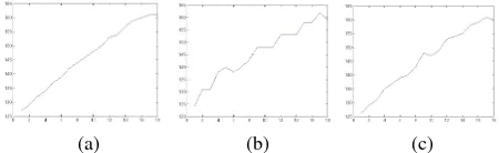
usually observed in photogrammetric DSMs on noisier areas; a parameter keeping in count this aspect is set to increase costs of displacements on higher labels. between adjacent points. For this reason, it properly smooth flat areas, where the label differences between adjacent points must be flatted. On slant surfaces like roofs (Figure 1a), the smoothing allows to completely delete gross errors, but it has the drawback to generate “artificial” steps on that surfaces (staircasing effect), making steep and flat segments alternated together, as shown in Figure 1b.
Assuming that roofs are mainly composed of local flat surfaces, an additional constraint should be considered in order to preserve their slope. A transition between different labels on adjacent points must be assured in a smoother way when points on a slant surface are considered (Figure 1c). Given the local inclination of the roof, the label of p could be predicted (Lpred) from surrounding point positions and an additional parameter can be added to the solution.
(a) (b) (c) Figure 1: ground truth (a) smoothing without (b) or using (c) Ssl
feature on a small DSM section.
(((( )))) ((((
(((( ))))
))))
(((( ))))
where α defines the inclination of the tilted surfaces:
Neighbourhood index (Cnp): each point is connected to
8-neighbouring points. Points in correspondence of unreliable areas are only connected to reliable points: in each of the eight directions the first reliable point is considered as neighbour. Assuming that points should be locally consistent, a point would have height values similar to (one or more) neighbouring points (Lneigh). In the same way, an unreliable point p should have a label close to reliable points. An additional parameter is added for unreliable points when labels close to neighbouring solutions close to neighbouring points.
All the features are integrated in the following data term maximum value is usually set to limit very high costs: the range is usually between 0 and 10. The adopted solution works with integer data term values: for this reason, Dp(lp) is approximated to the upper integer value.
In general, ∆L defines that the cost increases for labels that are far from the initial position of point p. The displacement to lower labels are advantaged by Cd and the cost increases faster on points considered as reliable than on unreliable points thanks to Ism. On unreliable points, labels corresponding to neighbouring points are enforced by Cnb. Finally, Ssl shifts the minimum cost in the direction of the predicted solution only on slanted surfaces.
The solution is influenced by the estimation of local smoothness of the point cloud defined by λ as most of the additional costs or the reductions are dependent from the estimated of the local smoothness of each point. Anyway, from the performed tests, the solutions has shown to be insensitive to moderate variations of λ providing very similar results.
4. PERFORMED TESTS
Several tests have been performed on the algorithm in order to tests its performances. Both synthetic and real images have been considered. In the following some of the achieved results are shown.
4.1 Synthetic DSM
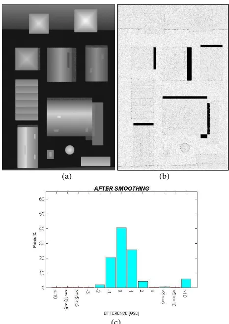
The synthetic 2.5D DSM was created using an image editor. The height values are provided by the grey values. Depth was defined in order to create simple but meaningful buildings able to simulate a real scenario. Roofs of different dimensions and shapes have been considered in order to evaluate the performance of the algorithms (Figure 2a).
(a) (b) Figure 2: ground truth (a) and noisy DSM (b). Then, additional noise has been added on the whole DSM as it is shown in Figure 2b:
- ±2 GSD of random depth noise to simulate the random noise of a photogrammetric DSM. The noise was in both upper and lower directions;
- Outliers have been added around some roof sides, on the ground or on adjacent buildings, to simulate gross errors due to occlusions and shadows. These outliers are randomly determined with a maximum amplitude of 40 GSD; the gross errors are in both upper and lower directions, but the outliers in the higher direction are bigger and mostly above the ground height.
- 10000 outliers spatially distributed and isolated: they simulate the matching outliers that can be found on the DSM. Their position is randomly generated, but they have maximum amplitude of ±10 GSD.
- Some mixed pixels: these points are in correspondence of the building borders, and they represent points with height between the roof and the ground.
All these noise has been added to the original DSM in order to evaluate the capability of the developed algorithm to reduce and recover the noise.
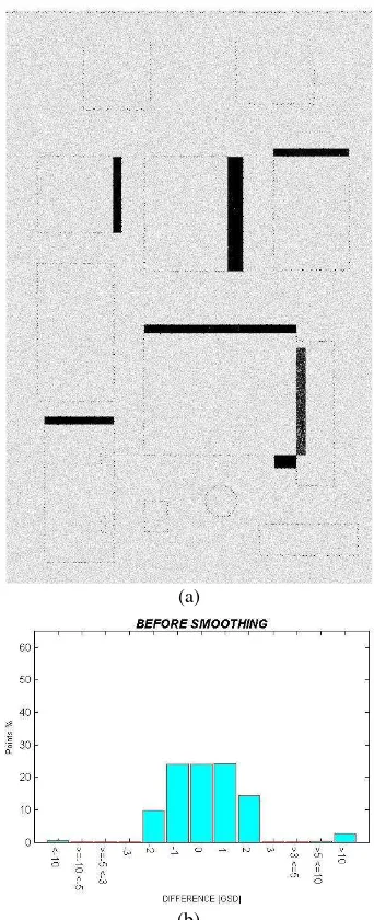
In Figure 3a, the differences between the ground truth and the noisy DSMs are presented. The white parts represent the areas where the two DSMs are coincident. The greyish colours represent points with differences that are comprised between 1 and 10 GSD: grey values ranges between 1 GSD of difference (brighter colours) to 10 GSD (darker colours). Differences larger than 10 GSD are represented in black. Finally, the differences (defined in GSD) and their relative frequencies are
reported in the histogram in Figure 3b. The histogram gives a global statistics on the remaining degradation. In practice such charts, however, do not sufficiently reflect the performance of an algorithm: local problems might still remain undetected. In this context the visualisation is very helpful: on the first sight one can see where a certain method fails.
(a)
(b)
Figure 3: differences between ground truth and noisy DSM (a) and histogram of the differences expressed in GSD (b). As it is possible to see from figure 3b points position is almost equally distributed in a range of ±2 GSD from the correct position and outliers are mainly distributed on the higher extreme.
In the following the results achieved using the described algorithms will be shown.
- Median Filter: the median filter reduces the random noise as it is shown by the histogram distribution; residuals are homogeneously distributed all over the DSM. Anyway, large noisy areas around buildings still persist and their amplitude is not changed appreciably (Figure 4). It is more the other way around: the fine roof structures on the building at the left border, centre area, do get enhanced.
(a) (b)
(c)
Figure 4: denoised DSM (a), differences between ground truth and the smoothed DSM using the median filter (b) and
histogram of the differences (c).
- Bilateral filter: the bilateral filter (the OpenCV libraries were used to implement this algorithm) was able to efficiently smooth the flat surfaces like the ground, but shows still high random noise residuals on the slanted surfaces. The gross errors are still visible and they are not reduced. In Figure 5a, 5b these results are reported. Some artefacts and medium differences (between 3 and 10 GSD) are generated on edges of the buildings and they are more evident in the histogram (Figure 5c).
(a) (b)
(c)
Figure 5: denoised DSM (a), differences between ground truth and the smoothed DSM using the bilateral filter (b) and
histogram of the differences (c).
- TGV regularization: The TGV filtering was used adopting the implementation available on the web and provided by (Getreuer, 2012). The TGV regularization algorithm was able to properly filter the random noise on the surfaces (Figure 6a, 6b) and a higher percentage of correct points (compared to the former methods) was achieved (Figure 6c). Anyway, the smoothing effect did not preserve the shape of the point cloud in correspondence of the building edges, where larger differences are visible (Figure 6a, 6b). Finally, it was not able to retrieve the correct position of large noisy regions around buildings.
(a) (b)
(c)
Figure 6: denoised DSM (a), differences between ground truth and the smoothed DSM using the TGV regularization filter (b)
and histogram of the differences (c). The International Archives of the Photogrammetry, Remote Sensing and Spatial Information Sciences, Volume XL-3, 2014
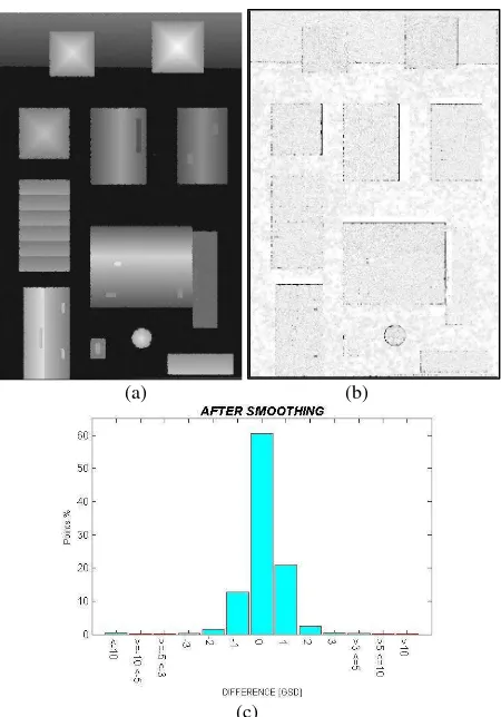
(a) (b)
(c)
Figure 7: denoised DSM (a), differences between ground truth and the smoothed DSM using the proposed algorithm (b) and
histogram of the differences (c).
- Proposed algorithm: the de-noising allows to remove almost completely the noisy regions around building and to retrieve the correct position of points. Some problems are still visible in correspondence of building edges, where some pixels are sometimes eroded and their height values can be sometimes underestimated.
The mean level of random noise of the DSM is greatly improved as shown in Figure 7a, b, where usually lighter grey colours are visible. This analysis is confirmed by the differences in Figure 7c, where more than the 90% of the DSM are concentrated in the error interval ±1 GSD: only where few points exceed this interval.
4.2 Real photogrammetric DSM
The DSM of the town of Transacqua (Italy) was generated using images acquired by a consumer grade single lens reflex camera (installed on an helicopter). 80% along track overlaps and 60% across track overlaps have been adopted in the flight; the DSM was generated using the MicMac software (IGN, France) and it has 18 cm of GSD. In the original point cloud, several outliers are visible, mainly due to building shadows and occlusions, while some noisy regions can be detected on the roof surfaces. A ground truth is not available, anyway a qualitative evaluation of the DSM before and after the DSM denoising can be performed to assess the effectiveness of the developed algorithm.
In Figure 8, the orthophoto of the analysed areas, the shaded visualization of the DSM before (Figure 8b) and after the denoising process are presented (Figure 8c).
The developed algorithm allowed to improve the results in correspondence of building borders. Black regions around buildings in Figures 8b describe the noisy area of the DSM: the dark colour is due to the rough height variations of the DSM. These areas appear strongly reduced in Figures 8c and gross errors are efficiently recovered in most of the cases. Points on noisy areas are usually moved on the ground by the algorithm. Isolated wrong points on the roof surfaces are correctly retrieved. Random noise is reduced on the roofs surfaces.
5. CONCLUSIONS AND FUTURE DEVELOPMENTS
Photogrammetric DSM are usually affected by both random noise and gross errors. These errors are generally concentrated in correspondence of occluded or shadowed areas and are strongly influenced by the texture of the object that is considered, or the number of images employed for the matching.
In this paper, different denoising methods have been evaluated to retrieve the correct point positions and deliver accurate point clouds. In particular, the effectiveness of common and a newly developed method to manage both these problems has been assessed.
To do that, a synthetic DSM, reproducing a realistic urban environment has been first generated. Different errors have been introduced to reproduce some typical errors that can be commonly detected on real DSM: the noise level, before and after the denoising process has been assessed using the algorithms, performing a quantitative evaluation.
The performed tests have shown that standard methods (median, bilateral smoothing, TGV-based) are only able to reduce the random noise problems, but they do not efficiently manage the presence of large noisy areas around buildings, and building corners get smoothed.
On the other hand, the developed algorithm based on MRF formulation has shown to provide better results both on random noise and gross error reduction: few remaining errors are mainly concentrated on the buildings borders. The algorithm uses as input a DSM and exploits few assumptions about the shape of the man-made objects and the height error distribution to set up an effective cost function. Tests on a real DSM have also confirmed the good performances of the algorithm at least from a qualitative point of view showing the ability of the presented methodology to reduce the noise on the building borders. The use of this prior information can strongly enhance the performance of the denoising process; on the other hand, it could limit the performance of the smoothing when unconventional errors patterns have to be recovered.
Another disadvantage of this method is the possibility to get stuck in local minima since the data term is not convex. Anyway, for the denoising application this problem is a minor drawback since a good initialization, the noisy DSM, is always available.
In the future, further tests will be performed on other real DSM in order to assess the reliability of the developed method in very different operative conditions. Then, the extension from the 2.5D case to the fully 3D will be performed and further comparisons with other available denoising algorithms will be performed, as well.
a)
b)
c)
Figure 8: Qualitative comparison of real case: the true ortho-photo of the area (a), the DSM before (b) and after (c) denoising.
ACKNOWLEDGEMENTS
We used the TGV implementation provided in
http://www.mathworks.nl/matlabcentral/fileexchange/29743-tvreg-variational-image-restoration-and-segmentation and
described in (Getreuer, 2012) and the graph cut implementation provided by http://vision.csd.uwo.ca/code/ and described in (Boykov and Komogorov, 2004).
REFERENCES
Ardila Lopez, J. P., Tolpekin, V. A., Bijker, W., Stein, A., 2011. Markovrandom-field-based super-resolution mapping for identification of urban trees in VHR images. In: ISPRS Journal of Photogrammetry and Remote Sensing 66 (6), pp. 762-775. Bae E., Shi, J., Tai, X.C., 2011. Graph-cuts for curvature based image Denoising. In: IEEE Transactions on image processing, 20(5), pp.1199-1210.
Boykov, Y., Kolmogorov, V., 2004. An Experimental Comparison of Min-Cut/Max-Flow Algorithms for Energy Minimization in Vision, In: IEEE Transactions on PAMI, 26(9), pp. 1124-1137.
Boykov, Y., Veksler, O., Zabih, R., 2001. Fast approximate energy minimization via graph cuts. In: PAMI 23 (11)
Cremers, D., Pock, T., Kolev, K., Chambolle, A., 2011. Convex relaxation for Segmentation, Stereo and Multiview Reconstruction. In: Chapter in Markov Random Fields for Vision and Image Processing, MIT Press, pp.1-24.
Digne, J., 2012. Similarity based filtering of point clouds. Proc. of: CVPR2012, online paper.
Furukawa, Y., Ponce, J., 2010. Accurate, dense and robust multiview stereopsis. In: IEEE Trans. PAMI, 32(8) pp. 1362-1376
Gerke, M. and Xiao, J., 2014. Fusion of airborne laserscanning point clouds and images for supervised and unsupervised scene The International Archives of the Photogrammetry, Remote Sensing and Spatial Information Sciences, Volume XL-3, 2014
classification. In: ISPRS Journal of Photogrammetry and Remote Sensing, 87, pp. 78-92.
Getreuer, P., 2012. Rudin–Osher–Fatemi Total Variation Denoising using Split Bregman, Image Processing. Online. DOI: 10.5201/ipol.2012.g-tvd, accessed April 6, 2014.
Haala, N., 2013. The landscape of dense image matching algorithms. Proc. of: Photogrammetric Week 2013. Wichmann Verla, Berlin/Offenbach, pp. 271-284.
Hirschmüller, H., 2008. Stereo processing by semi-global matching and mutual information. IEEE Trans. PAMI, Vol. 30(2), pp. 328-341.
Li, S. Z., 2009. Markov random field modeling in image analysis, 3rd Edition. Advances in Computer Vision and Pattern Recognition. Springer, Berlin.
Meixner, P., Leberl, F., Brédif, M., 2011. Prof of: 19th ACM SIGSPATIAL International Conference on Advances in Geographic Information Systems, pp. 9-15.
Perona, P., Malik, J., 1990. Scale-space and edge detection using anisotropic diffusion. In: IEEE Transactions on Pattern Analysis and Machine Intelligence, 12(7) pp. 629–639.
doi:10.1109/34.56205.
Pierrot-Deseilligny, M. and Paparoditis, N., 2006. A multiresolution and optimization-based image matching approach: An application to surface reconstruction from Spot5-HRS stereo imagery. ISPRS Int. Archives of Photogrammetry, Remote Sensing and Spatial Information Sciences, Vol. 36(1/W41).
Pock T., Zebedin, L., Bischof, H., 2011. TGV-Fusion In: C.Calude, G. Rozenberg, A. Salomaa (Eds.), Rainbow of Computer Science, in: Lecture Notes in Computer Science, Vol. 6570, Springer, Berlin, Heildelberg, pp. 245-258.
Remondino, F., Spera, M.G., Nocerino, E., Menna, F., Nex, F., Gonizzi-Barsanti, S., 2013. Dense image matching: comparisons and analyses. Proc. of: Digital Heritage International Conference, Vol. 1, pp. 47-54 ISBN 978-1-4799-3169-9.
Tomasi, C., Manduchi, R., 1998. Bilateral Filtering for Gray and Color Images. Proc. of: 6th International Conference on Computer Vision (ICCV ’98). IEEE Computer Society, Washington DC.
Yan, D., Yongzhuang, M., 2007. Image restoration using graph cuts with adaptive smoothing.