TO EXAMINE THE ASSOCIATION BETWEEN OSCILLATIONS OF THE
STRATOSPHERIC AEROSOL LAYER PEAKS AND DIFFERENT TYPES OF
CLOUDS
Pratibha B. Mane
Department of Physics, Shivaji University, Kolhapur-416 004, Maharashtra state, India. [email protected]
KEY WORDS: aerosols; Aerosol Number Density; twilight photometer; clouds; Junge layer; passive remote sensing
ABSTRACT: Aerosol measurements have been carried out at Kolhapur (16°42′N, 74°14′E) by using newly designed Semiautomatic Twilight Photometer. The system is a ground based simple and inexpensive but very sensitive passive remote sensing technique. The altitudes of the Junge layer peaks on measurement days were derived from the aerosol vertical profiles. One attempt is made to examine the association between oscillations of the stratospheric aerosol layer peaks and different types of clouds. The values of AND for the Junge layer peaks for each observational day were also calculated. The graph between AND at peak point of Junge layer and day numbers was also studied in comparison with High, Medium and Low level clouds. There is an annual variation in the altitude of the peak of Junge layer also. Its maximum is observed during January. The annual variation of the altitude of the peak of Junge layer and the AND of Junge layer peak showed opposite phase relation.
1. INTRODUCTION
Atmospheric aerosols are the suspension of fine solid particles or liquid droplets in air. Depending upon the source size of aerosols varies from 10-3 to 102μm. Particles larger than 100 μm cannot remain suspended in air for long periods. Dust, smoke, mist, fog, haze and smog are various forms of common aerosols. Aerosols are of considerable interest in atmospheric sciences. This is mainly due to their potential of changing the radiative transfer of solar radiation as a direct influence, and due to the complex indirect consequences connected with aerosol induced cloud and precipitation processes. These two processes essentially determine the earth's climate. Aerosols are closely related to the atmospheric chemistry and atmospheric electrical conductivity. The consequences arising from an increased aerosol concentration remain extremely difficult to understand because vertical distribution of aerosols is strong function of their sources, sinks and their residence times. Aerosols are distributed in the different atmospheric levels. The sources, sinks and characteristics of aerosols in the different atmospheric levels are markedly different. Aerosols affect the progress of twilight, as more the number of aerosols in the atmosphere, more the sky brightness during the twilight period.
Aerosols, the giant particles (Coarse mode- >1 m) are of major importance in the nucleation and cloud formation processes. Clouds with more CCN are larger and more reflective than those with fewer CCN, so they also add to cooling in the atmosphere. Cloud formation is dependent on aerosols. If no aerosols are present, large super-saturation (relative humidity over 100%) can be observed without droplet formation. But small particles, in different concentrations, are present everywhere in the atmosphere. Cloud droplets condense on the aerosols. If few particles (less than 200 per cm3) are available as cloud condensation nuclei, large droplets are formed. If a large number of aerosols are present, smaller droplets are formed. Clouds with large droplets reflect sunlight less effectively compared to clouds with small droplets. Clouds effectively reflect solar radiation and low clouds contribute particularly to a cooling effect. However, high, wispy cirrus clouds that can have relatively large droplets, do not reflect solar light very effectively, but will almost completely reflect long wave infrared radiation. The reduction of cloud droplet
size with increasing number of aerosol particles is not linear. It is quite important at low particle numbers (under clean conditions, 100 particles per cm3) but increasing particle number over 1,000 particles per cm3 no longer has any effect
The stratospheric aerosols are studied by several workers in all over the world (Jadhav et. al.2000). In the present work aerosol measurements have been carried out at Kolhapur (16°42′N, 74°14′E) by using newly designed Semiautomatic Twilight Photometer during the period 1 January 2009 to 30 December 2011 to study the vertical distribution of the stratospheric aerosol number density per cm3 (AND) (Here after aerosol number density per cm3 is abbreviated as AND). This is being a passive technique; clear sky conditions are preferable for obtaining the vertical profile of aerosols. The days on which low, middle and high level clouds were observed also noted down during the period of observations. Kolhapur city, a location in the south-waste Maharashtra is selected for this study because this station is free from any large scale industrial and urban activities or biomass burning and also surrounded by agricultural land mainly. It has an elevation of 569 meters. It is having blend of coastal and inland climate of Maharashtra.
The stratospheric aerosol layer was first measured in the late 1950s using balloon-borne impactors (Junge et.al 1961a and Junge et. al. 1961b) and is often called the Junge layer, although its existence was suggested 50 years earlier from twilight observations (Gruner et. al. 1927). These particles are composed of sulfuric acid and water and are formed by the chemical transformation of sulfur-containing gases. By screening out sunlight, the Junge layer affects the atmospheric energy balance and hence climate. The layer can also alter chemical cycles and perturb ozone levels. The stratospheric aerosol layer is sustained by natural emissions of carbonyl sulfide (OCS) through biogenic processes. Carbonyl sulfide is relatively stable can mix into the stratosphere where it is photo chemically broken down resulting in the formation of microscopic droplets of sulfuric acid. Another sulfur-containing gas, sulfur dioxide (SO2), is normally too reactive to reach the stratosphere; instead it is rained out (as acid rain downwind of its sources). Volcanic eruptions, however, can inject SO2 directly into the stratosphere where it too undergoes transformation into sulfuric acid. But most volcanic eruptions do not penetrate into the stratosphere. In fact only a small number of eruptions in this century have had a significant impact on the Junge Layer. The most recent example is the June 1991 eruptions of Mt. Pinatubo .
In the present study the altitudes of the Junge layer peaks on measurement days were derived from the aerosol vertical profiles. These altitudes were used to calculate oscillations of the Junge layer peaks on consecutive days. One attempt is made to examine the association between oscillations of the stratospheric aerosol layer peaks and different types of clouds. The values of AND for the Junge layer peaks for each observational day were also calculated. The graph between AND at peak point of Junge layer and day numbers was also studied in comparison with different types of clouds.
The clouds are classified according to height of cloud base. Thus clouds are mainly divided into three groups:
i. High level clouds: The bases of high level clouds lie between ~6 km and ~12 km. These types of clouds include cirrus clouds, cirrocumulus clouds and cirrostratus clouds. Contrails are also one type of high level clouds.
ii. Medium level clouds: The bases of medium level clouds lie between ~2 km and ~6 km. These types of clouds include altocumulus clouds and altostratus clouds.
iii. Low level clouds: The base of low level clouds lie below 2 km. These types of clouds include nimbostratus clouds and stratocumulus clouds. Fog is also one type of low level cloud in contact with ground.
2. ISTRUMENTATION
The instrument, semiautomatic twilight photometer, is newly designed, developed and tested at Shivaji University, Kolhapur, Maharastra, India. The system is a ground based passive remote sensing technique used to monitor the vertical distribution of the atmospheric aerosols. It is a simple and inexpensive but very sensitive technique and hence can be operated continuously for monitoring the day-to-day variability of the aerosols, at any place. The twilight photometer setup operated manually is used by several workers in all over the world (Jadhav et. al.2000). However, during the course of this study the system is suitably modified to improve the sensitivity of the system.
The semiautomatic twilight photometer consists of a simple experimental set up. It comprises of a pleno-convex lens of diameter 15 cm having a focal length of 35 cm. A red band pass glass filter peaking at 670 nm with a half band width of about 50 nm is used. The red filter of 1.2 cm diameter and an aperture of 0.6 cm diameter are placed at the focal length of convex lens, provides approximately 10 field of view [(Aperture diameter/Focal length of lens) X57= (0.6cm/35cm) X 7=0.9771 degree]. A photomultiplier tube (PMT-9658B) is used as a detector. The PMT requires high voltage supply (700 V). The output signal (current) of the PMT, used for detecting the light intensity during the twilight period, is very low. It is of the order of nano to microamperes. The amplitude or strength of this low signal is amplified by using a newly designed fast pre-amplifier. The more details regarding the instrument and Fast pre-amplifier were given elsewhere, (Mane et al., 2012a and Mane et al., 2012b). The amplifier output recorded by the digital multimeter, Rishcom-100, having an adapter can store the data automatically for every 10 seconds in the form of date, time and intensity in Volts. During evening, the twilight photometer is operated for a time spell of ~90 minutes after the local sunset and during morning it is operated ~90 minutes before the sunrise.
Some noticeable features of the Semiautomatic Twilight Photometer are: Augmented efficiency of the system, Improvement in height resolution, Increased duration of operation of the system, Visibility of the small fine-scale features in the profiles derived by this system, A lot of upgrading in the sensitivity of the system, Amplified Signal to noise ratio, Drastically reduction in the white noise of the system, Better accuracy in measurement and recording the data, Amplified Signal to noise ratio. Hence it is able to give the information of aerosols in the atmosphere up to higher altitudes (from 6 km to 350 km).
3. BASIC PRINCIPLE OF TWILIGHT TECHNIQUE
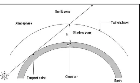
Following Figure-1 shows the twilight phenomenon schematically.
Figure 1: Schematic diagram of twilight phenomenon
the light scattered by illuminated by molecules and the particles of interest. It is assumed that bulk of the scattered light comes to an observer from the lowest, and therefore densest, layer in the sunlit atmosphere at the time of measurement. The contribution of the rest of the atmosphere above this layer can be neglected due to an exponential decrease of air density with increasing altitude. The height of this lowest layer (twilight layer) increases with increasing earth's shadow height. The lower atmospheric layers now submerged in shadow, no longer contribute to the sky brightness, and the scattered light comes more and more from the higher altitudes, which are still illuminated by direct sunlight.
The method for calculating the earth's geometrical shadow height (h) is given by Shah (1970). Thus the earth's geometrical shadow height (h) is defined as the vertical height from the surface of the earth, of a point where the solar ray grazing the surface of the earth meets the line of slight. Therefore,
h = R (sec [ ] - 1) ... (1)
Where, R is radius of earth and is sun's depression.
In following the method of Shah (1970), it is assumed that the red twilight comes from a distance of 6 Km. The raw data consists of intensity ‘I’ and time ‘t’. The shadow heights were computed for zenith sky observations, and the raw data was utilized for the analysis of ‘1/I (dI/dh)’ value, where ‘I’ is the observed intensity, ‘dI’ and ‘dh’ are the differences in intensities and shadow heights respectively observed at time ‘t’ and ‘t+dt’.
As the sun sinks below the horizon, the effective height of the Earth’s shadow rises and scattering takes place to higher levels. Most of the light received at the ground will be the primary scattered light by the particles for the solar depression less than 6-7 deg (Shah, 1970). Therefore,
The effect of the Rayleigh scattering component on the value of ‘1/I (dI/dh)’ has been studied by Bigg (1956). Variations in the vertical profiles of the molecular density were very small and their effect on the observed intensity was nearly constant, hence the variations in the value of – (1/I) (dI/dh) can be assumed to be mainly due to changes in aerosols density. Thus,
Logarithmic gradient of the intensity cannot give the information about the aerosol number density. Therefore an empirical formula stated in equation-4 is derived by the actual Lidar observations and the Photometric observations. Thus,
Aerosol number density per cm3 (AND) =
Antilog10{10[‘1/I (dI/dh)’]-1} ….. (4)
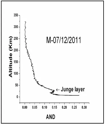
One of the aerosols vertical profiles in terms of AND is as shown in the following Figure-2. It is clear from this figure that
the value of AND decreases with height in troposphere. In the lower stratosphere, the value of AND increases slightly due to the presence of stratospheric dust layer, also called as Junge layer. After that, the value of AND decreases as the altitude increases (Mane, 2013).
Figure 2: Aerosol vertical profiles in terms of AND
4. RESULTS AND DISCUSSION
4.1. Comparison between altitude of Junge layer peaks and cloudy days
Figure-1: Comparison between altitude of Junge layer peaks and cloudy days
The graph was studied carefully and results were noted. The results acquired reveal that:
I. The altitudes of junge layer peaks for clear sky days showed day to day, monthly and seasonal variations.
II. In the month of October the junge layer peak was at ~12 km and increases slowly up to January. It lies between ~ 18 to 23 km in the month of January and decreased slowly up to ~15 km for the month of April.
III. The Post-monsoon (from October to November) and summer or Pre-monsoon (from March to May) seasons shows lower altitudes of junge layer peaks; while it was at higher altitudes in winter season (from December to February).
IV. The sky was almost clear in January and March. In October, November, December and February all the three types of clouds observed frequently. Observational information shows some relation between the oscillations of altitudes of Junge layer peaks and occurrences of different types of clouds.
V. High-level clouds: The altitude of Junge layer peak for clear sky day, preceding the high level cloudy sky day lowered down to ~11 km and increased up to ~19 km on the clear sky day following the high level cloudy sky day. The some
examples of high level cloudy days were 11 February (day number-107), 16 February (112), 14 March (137) and 29 October (2). It implies that the aerosols slide down acts as the cloud condensation nuclei (CCN).
VI. Medium and low level clouds: Middle and low level clouds were frequently observed following with high level clouds. In very rare cases middle level cloudy days were noticed separately after any clear sky day. The altitude of Junge layer peak suddenly decreased up to ~11 km at two days before the low level clouds observed day. For example 23 February 2011 (day number 119) is the low-level cloudy day; while the altitude of Junge layer peak suddenly decreased up to ~10.98 km at 21 February 2011 (day number 117).
VII. Fog or dew drops: In winter the altitude of Junge layer peak decreased at three days prior to the days on which fog or dew drops were observed.
4.2. Comparison between AND of Junge layer peaks and cloudy days
The aerosol number density per cm3 (AND) for peak point of the Junge layer was also calculated for every clear sky day. A graph between AND at peak point of Junge layer and day numbers was also plotted. High, medium and low level cloudy days also noted down and they were included in this graph also. The graph between AND at Junge layer peak point and day numbers was shown in the Figure-4. The black line in this graph corresponds to the AND of Junge layer peak for clear sky days. In this graph Y-axis represents AND of Junge layer peaks and X-axis stands for day numbers. The day number 1 corresponds to 28 October 2010; 65 correspond to 31 December 2010; 66 to 185 correspond to 1 January 2011 to 30 April 2011.
The graph was studied carefully and results were noted. The results acquired reveal that:
I. The AND of junge layer peaks for clear sky days showed day to day, monthly and seasonal variations.
II. In the month of October the AND of junge layer peak was ~10-12 particles/cm3 and increases slowly up to January. It lies between ~4-6 particles/cm3 in the month of January and increased slowly up to ~7-8 particles/cm3 for the month of April.
III. The Post-monsoon (from October to November) and summer or Pre-monsoon (from March to May) seasons shows Higher values of AND for junge layer peaks; while it was at lower altitudes in winter season (from December to February).
IV. The annual variations of the altitudes of the peaks of Junge layer and the AND of Junge layer peaks showed opposite phase relation.
V. The sky was almost clear in January and March. In October, November, December and February all the three types of clouds observed frequently. Observational information shows some relation between the oscillations of AND of Junge layer peaks and occurrences of different types of clouds.
VI. High-level clouds: The AND of Junge layer peak increased near about two times at two days before the high level cloudy sky day and decreased up normal values on the clear sky day following the high level cloudy sky day. The some examples of high level cloudy days were 11 February (day number-107), 16 February (112), 14 March (137) and 29 October (2). It implies that the aerosols slide down acts as the cloud condensation nuclei (CCN).
VII. Medium and low level clouds: Middle and low level clouds were frequently observed following with high level clouds. In very rare cases middle level cloudy days were noticed separately after any clear sky day. The value of AND of Junge layer peak suddenly increased too much (three times the normal values) at two days before the low level cloudy day. For example 23 February 2011 (day number 119) is the low-level cloudy day; while the AND of Junge layer peak suddenly increased at 21 February 2011 (day number 117).
VIII. Fog or dew drops: In winter the AND of Junge layer peak increased nearly four times at three days prior to the days on which fog or dew drops were observed.
From the above two curves it was expected that the aerosol layer with increased quantity of aerosols would come down to a lower altitudes to create favorable conditions for cloud development. The observational evidence supported this fact. However, at present the definite relation between oscillations of Junge layer peak and weather conditions could not be established with so few data events. But it is possible if a greater number of events are available.
Considering the seasonal variation of natural factors like temperature and rains Raju et al. (2000), explained the experimentally observed features of aerosol characteristics as follows. The average temperature patterns for winter and summer months show significant differences. The relatively higher temperature in summer would result in enhanced aerosol generation due to primary production (bulk-to-particle conversion) and photochemical processes (secondary production) as compared to that in winter with low temperatures. During monsoon, the wet removal (scavenging) of atmospheric aerosols would be more efficient due to heavy and prolonged monsoon rains than in winter or summer seasons. The combined effect of significant wet removal of atmospheric aerosols in monsoon season, which precede the winter months, and the decreased production of small aerosols by secondary production in winter months result in an overall reduction of aerosols. In summer, there would be remarkable enhancement in the total aerosol load due to increased small particle concentration from secondary processes and large particles from primary production. In addition, the presence of substantial but infrequent rains in summer and almost total absence of rains in winter months would influence the generation, growth and loss processes of the aerosols. Further, the usual dry conditions with reduced humidity in winter months and comparatively high humidity in summer months would affect the coagulation and growth processes of aerosols in winter and summer months. Thus the observed seasonal variations in the AND (in the present study) are as a result of the natural variations in the production and removal of aerosols in summer and winter. The experimental results obtained by the present study are well agreement with theory.
Nighut et.al. (1999), suggested that the aerosol layer maxima shows downward drifting before cloudy days and upward drifting after cloudy days. The results obtained by present study are very well matching with the results obtained by Nighut et.al. (1999). Many of the consequences of present paper are in good agreements with the conclusions reveal by Jadhav and Londhe (1992).
4.3. Three years annual variations for altitudes of Junge layer peaks
Following Figure-5 shows three years annual variations for altitudes of Junge layer peaks. In this graph Y-axis represents altitude of Junge layer peaks and X-axis stands for day numbers. The day number 1 corresponds to 1 January and 365 correspond to 31 December for each year. The black line represents annual variations of altitude of Junge layer peaks from 1 January 2009 to 31 December 2009; red line from 1 January 2010 to 31 December 2010 and green line from 1 January 2011 to 31 December 2011. For every year observations stop at mid of May and start at mid of October. Thus no data available from mid of May to mid of October. Hence the graph is split in to two parts; one from January to mid of May and another from mid of October to December for each year.
The Junge layer peaks observed at higher altitudes (nearly two times) for year 2010, in the months from January to May than 2009. There was ~ 50% increase in the altitudes of the Junge layer peaks for year 2011, in the months from mid of January to mid of April than 2009. The months October to December showed no altitudinal variations for all the three years.
Figure-5: Three years annual variations for altitudes of Junge layer peaks
4.4. Three years annual variations for AND of Junge layer peaks
Following Figure-6 shows three years annual variations for AND of Junge layer peaks. In this graph Y-axis represents AND of Junge layer peaks and X-axis stands for day numbers. The day number 1 corresponds to 1 January and 365 correspond to 31 December for each year. The black line represents annual variations of AND of Junge layer peaks from 1 January 2009 to 31 December 2009; red line from 1 January 2010 to 31 December 2010 and green line from 1 January 2011 to 31 December 2011. For every year observations stop at mid of May and start at mid of October. Thus no data available from mid of May to mid of October. Hence the graph is split in to two parts; one from January to mid of May and another from mid of October to December for each year.
The values of AND for Junge layer peaks showed no considerable difference in the months of October, November, December, January and May. The months from February to April revealed lower values of AND for the year 2010. The month of February showed ~ 25% variation, March showed ~55% difference and April showed ~ 65% deviation for the values of AND in between the years 2009 and 2010. The month of February showed no variation, March showed ~ 30% difference and April showed ~55% deviation for the values of AND in between the years 2009 and 2011.
5. SUMMARY AND CONCLUSIONS
The measurements using the ‘twilight sounding method (TSM)’ presented in this paper suggest the following,
I. The AND of junge layer peaks and its altitudes for clear sky days showed day to day, monthly, seasonal and annual variations.
II. The annual variation of the altitude of the peak of Junge layer and the AND of Junge layer peak showed opposite phase relation.
III. It will be possible to establish the definite relation between oscillations of the stratospheric aerosol layer peaks and weather conditions including different types of clouds, if a greater number of events are available.
IV. The continuous and detail study of Junge layer for some years, will able to give precursor for different types of clouds.
V. The results of the present study are mostly speculative and to arrive at significant result greater numbers of sets of observations are essential.
Acknowledgements: Author is grateful to the Shivaji University authorities, Kolhapur, for the encouragement during the course of this work and also the SERB, DST, India, for providing funds through the Fast Track Scheme for Young Scientists Fellowship for the development of twilight photometer.
REFERANCES
1. Bigg, E. K., 1956. The detection of atmospheric dust and temperature inversion twilight scattering. Journal of Meteorology, 13, 262-268.
2. Crutzen, P. J. 1976. The possible importance of CSO for the sulfate layer of the stratosphere. Geophy. Res. Lett., 3, 73-76.
3. Fahey, D. W., Kawa, S. R., Woodbridge, E. L., Tin, P., Wilson, J. C., Jonsson, H. H., Dye, J. E., Baumgardner, D., Borrmann, S., Toohey, D. W., Avallone, L. M., Proffitt, M. H., Margitan, J., Loewenstein, M., Podolske, J. R., Salawitch, R. J., Wofsy, S. C., Ko, M. K. W., Anderson, D. E., Schoeber, M. R., and Chan, K. R.1993. In situ measurements constrainting the role of sulphate aerosols in mid-latitude ozone depletion. Nature, 363, 509–514, doi: 10.1038/363509a0.
4. Gruner, P. & H. Kelinert, 1927. Die Dammerungser schcinugen, Problem der Kosmischen physik, 10, herri Gand, Hamburg.
5. Jadhav D. B., B. Padma Kumari & A. L. Londhe, 2000. A review on twilight photometric studies for stratospheric aerosols. Bulletin of Indian Aerosol Science & Technology Association, 13, 1 – 17. 6. Jadhav, D. B. & A. L. Londhe, 1992. Study of
atmospheric aerosol loading using the twilight method. J. Aerosol Sci., 23, 623-630.
7. Junge, C. E. and Manson J. E., 1961. Stratospheric aerosol studies. J. Geophys. Res., 66, 2163-2182.
8. Junge, C. E., Changnon, C. W. and J. E. Manson, 1961. Stratospheric aerosols, J. Meteorol., 18, 81–108. 9. K¨archer, B., and Str¨om, J. 2003. The roles of
dynamical variability and aerosols in cirrus cloud formation. Atmos. Chem. Phys., 3, 823–838.
10. Mane Pratibha B., Jadhav D. B., A.Venkateswara Rao, 2012a. Semiautomatic twilight photometer design and working. IJSER, 3(7), 1-7.
11. Mane Pratibha B., Jadhav D. B., A.Venkateswara Rao, 2012b. Fast pre-amplifier designed for semiautomatic twilight photometer. DAV International Journal of Science, 1(2), 9-11.
12. Mane Pratibha B., 2013. To Reveal the Aerosol Vertical Profiles in Terms of Aerosol Number Density. Indian Journal of Applied Research, 3 (12), 521-523.
13. Mc Cormick, M. P. & R. E. Vegia, 1992. SAGE II measurements of early Pinatubo aerosols. Geophys. Res. Lett.., 19, 155-158.
14. Nighut, D. N., A. L. Londhe, D. B. Jadhav, 1999. Derivation of vertical profile in lower stratosphere & upper troposphere using twilight photometry. Indian J. Radio & Space Phys., 28, 75-83.
15. Penner, J. E., Chen, Y.,Wang, M., and Liu, X.2009. Possible influence of anthropogenic aerosols on cirrus clouds and anthropogenic forcing. Atmos. Chem. Phys., 9, 879–896.
16. Raju N. V., B S N Prasad, B Narasimhamurthy and M Thukarama, 2000. Meteorological and anthropogenic influences on the atmospheric aerosol characteristics over a tropical station Mysore (120N). Indian J. Radio & Space Phys., 29 (3), 115-126.
17. Shah, G. M., 1970. Study of aerosol in the atmosphere by twilight scattering. Tellus, 22, 82-93.