and Cosmology
Ian Morison
University of Manchester, UK
and Cosmology
Ian Morison
University of Manchester, UK
Registered offi ce
John Wiley & Sons Ltd, The Atrium, Southern Gate, Chichester, West Sussex, PO19 8SQ, United Kingdom
For details of our global editorial offi ces, for customer services and for information about how to apply for permission to reuse the copyright material in this book please see our website at www.wiley.com.
The right of the author to be identifi ed as the author of this work has been asserted in accordance with the Copyright, Designs and Patents Act 1988.
All rights reserved. No part of this publication may be reproduced, stored in a retrieval system, or transmitted, in any form or by any means, electronic, mechanical, photocopying, recording or otherwise, except as permitted by the UK Copyright, Designs and Patents Act 1988, without the prior permission
of the publisher.
Wiley also publishes its books in a variety of electronic formats. Some content that appears in print may not be available in electronic books.
Designations used by companies to distinguish their products are often claimed as trademarks. All brand names and product names used in this book are trade names, service marks, trademarks or registered trademarks of their respec-tive owners. The publisher is not associated with any product or vendor mentioned in this book. This publication is designed to provide accurate and authoritative information in regard to the subject matter covered. It is sold on the understanding that the publisher is not engaged in rendering professional services. If professional advice or other expert assistance is required, the services of a competent professional should be sought.
The publisher and the author make no representations or warranties with respect to the accuracy or completeness of the contents of this work and specifi cally disclaim all warranties, including without limitation any implied warranties of fi tness for a particular purpose. This work is sold with the understanding that the publisher is not engaged in render-ing professional services. The advice and strategies contained herein may not be suitable for every situation. In view of ongoing research, equipment modifi cations, changes in governmental regulations, and the constant fl ow of informa-tion relating to the use of experimental reagents, equipment, and devices, the reader is urged to review and evaluate the information provided in the package insert or instructions for each chemical, piece of equipment, reagent, or device for, among other things, any changes in the instructions or indication of usage and for added warnings and precautions. The fact that an organization or Website is referred to in this work as a citation and/or a potential source of further information does not mean that the author or the publisher endorses the information the organization or Website may provide or recommendations it may make. Further, readers should be aware that Internet Websites listed in this work may have changed or disappeared between when this work was written and when it is read. No warranty may be cre-ated or extended by any promotional statements for this work. Neither the publisher nor the author shall be liable for any damages arising herefrom.
Library of Congress Cataloging-in-Publication Data Morison, Ian, 1943–
Introduction to astronomy and cosmology / Ian Morison. p. cm.
Includes bibliographical references and index.
ISBN 978-0-470-03333-3 (cloth) — ISBN 978-0-470-03334-0 (pbk. : alk.paper) 1. Astronomy—Textbooks. 2. Cosmology—Textbooks. I. Title.
QB43.3.M67 2008 520—dc22
2008029112 A catalogue record for this book is available from the British Library.
Preface xv
Biography xvii
Chapter 1: Astronomy, an Observational Science
1
1.1 Introduction 1
1.2 Galileo Galilei’s proof of the Copernican theory of the solar system 1 1.3 The celestial sphere and stellar magnitudes 4
1.3.1 The constellations 4
1.3.2 Stellar magnitudes 5
1.3.3 Apparent magnitudes 5
1.3.4 Magnitude calculations 6
1.4 The celestial coordinate system 7
1.5 Precession 9
1.6 Time 11
1.6.1 Local solar time 11
1.6.2 Greenwich mean time 11
1.6.3 The equation of time 12
1.6.4 Universal time 12
1.6.5 Sidereal time 13
1.6.6 An absolute time standard – cosmic time 14 1.7 A second major observational triumph: the laws of planetary motion 16 1.7.1 Tycho Brahe’s observations of the heavens 17 1.7.2 Johannes Kepler joins Tycho Brahe 20
1.7.3 The laws of planetary motion 20
1.8 Measuring the astronomical unit 23
1.9 Isaac Newton and his Universal Law of Gravity 25 1.9.1 Derivation of Kepler’s third law 30 1.10 Experimental measurements of G, the Universal constant
of gravitation 32
1.11 Gravity today: Einstein’s special and general theories of relativity 33
1.12 Conclusion 36
1.13 Questions 36
Chapter 2: Our Solar System 1 – The Sun
39
2.1 The formation of the solar system 39
2.2 The Sun 43
2.2.1 Overall properties of the Sun 43
2.2.2 The Sun’s total energy output 45
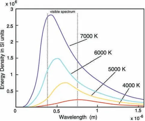
2.2.3 Black body radiation and the sun’s surface temperature 46 2.2.4 The Fraunhofer lines in the solar spectrum and the composition
of the sun 49
2.3 Nuclear fusion 50
2.3.1 The proton–proton cycle 53
2.4 The solar neutrino problem 57
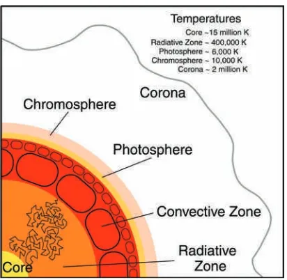
2.4.1 The solar neutrino problem is solved 58 2.5 The solar atmosphere: photosphere, chromosphere and corona 59
2.5.1 Coronium 61
2.6 The solar wind 61
2.7 The sun’s magnetic fi eld and the sunspot cycle 62
2.7.1 Sunspots 62
2.7.2 The sunspot cycle 64
2.8 Prominences, fl ares and the interaction of the solar wind with
the earth’s atmosphere 65
2.8.1 The aurora 66
2.9 Solar eclipses 67
2.9.1 Two signifi cant solar eclipses 69
2.9.2 The Shapiro delay 71
2.10 Questions 72
Chapter 3: Our Solar System 2 – The Planets
75
3.1 What is a planet? 75
3.2 Planetary orbits 77
3.2.1 Orbital inclination 78
3.3 Planetary properties 79
3.3.1 Planetary masses 79
3.3.2 Planetary densities 80
3.3.3 Rotation periods 80
3.3.4 Planetary temperatures 81
3.3.5 Global warming 83
3.4 Planetary atmospheres 84
3.4.1 Secondary atmospheres 86
3.4.2 The evolution of the earth’s atmosphere 87
3.5 The planets of the solar system 87
3.5.1 Mercury 88
3.5.2 Venus 89
3.5.3 The Earth 92
3.5.4 The moon 94
3.5.5 Mars 102
3.5.6 Ceres and the minor planets 106
3.5.7 Jupiter 108
3.5.8 Saturn 113
3.5.9 Uranus 117
3.5.10 Neptune 120
3.5.11 Pluto 124
3.5.12 Eris 128
3.6 Comets 129
3.6.1 Halley’s comet 130
3.6.2 Cometary nuclei 131
3.7 Questions 132
Chapter 4: Extra-solar Planets
135
4.1 The radial velocity (Doppler wobble) method of planetary detection 135
4.1.1 Pulsar planets 138
4.1.2 The discovery of the fi rst planet around a sun-like star 139
4.2 Planetary transits 142
4.3 Gravitational microlensing 145
4.4 Astrometry 148
4.5 Discovery space 149
4.6 Selection effects and the likelihood of fi nding solar systems like ours 151
4.7 Questions 151
Chapter 5: Observing the Universe
153
5.1 Thinking about optics in terms of waves rather than rays 153
5.1.1 The parabolic mirror 153
5.1.2 Imaging with a thin lens 156
5.2 The human eye 161 5.3 The use of a telescope or pair of binoculars to see fainter objects 163 5.4 Using a telescope to see more detail in an image 164
5.4.1 An interesting worked example of the effects
of diffraction 166
5.4.2 The effect of diffraction on the resolution of a telescope 167
5.5 The magnifi cation of a telescope 168
5.6 Image contrast 170
5.7 The classic Newtonian telescope 170
5.8 The Cassegrain telescope 172
5.9 Catadioptric telescopes 172
5.9.1 The Schmidt camera 172
5.9.2 The Schmidt–Cassegrain telescope 173 5.9.3 The Maksutov–Cassegrain telescope 174
5.10 Active and adaptive optics 174
5.10.1 Active optics 175
5.10.2 Adaptive optics 175
5.11 Some signifi cant optical telescopes 176 5.11.1 Gemini North and South telescopes 176
5.11.2 The Keck telescopes 177
5.11.3 The South Africa Large Telescope (SALT) 177 5.11.4 The Very Large Telescope (VLT) 178 5.11.5 The Hubble Space Telescope (HST) 179 5.11.6 The future of optical astronomy 180
5.12 Radio telescopes 181
5.12.1 The feed and low noise amplifi er system 182
5.12.2 Radio receivers 183
5.12.3 Telescope designs 184
5.12.4 Large fi xed dishes 186
5.12.5 Telescope arrays 188
5.12.6 Very Long Baseline Interferometry (VLBI) 189 5.12.7 The future of radio astronomy 191
5.13 Observing in other wavebands 193
5.13.1 Infrared 193
5.13.2 Submillimetre wavelengths 193
5.13.3 The Spitzer space telescope 195
5.14 Observing the universe without using electromagnetic
radiation 197
5.14.1 Cosmic rays 197
5.14.2 Gravitational waves 199
5.15 Questions 202
Chapter 6: The Properties of Stars
205
6.1 Stellar luminosity 205
6.2 Stellar distances 205
6.2.1 The parsec 207
6.3 Proper motion 208
6.3.1 Hipparcos and GAIA 208
6.4 The absolute magnitude scale 209
6.4.1 The standard formula to derive absolute
magnitudes 210
6.5 Colour and surface temperature 212
6.6 Stellar photometry 214
6.7 Stellar spectra 214
6.7.1 The hydrogen spectrum 215
6.7.2 Spectral types 216
6.8 Spectroscopic parallax 217
6.9 The Hertzsprung–Russell Diagram 219
6.9.1 The main sequence 220
6.9.2 The giant region 220
6.9.3 The white dwarf region 222
6.9.4 Pressure broadening 222
6.10 The size of stars 223
6.10.1 Direct measurement 223
6.10.2 Using binary star systems to calculate stellar sizes 225 6.10.3 Using the Stephan–Boltzman law to estimate
stellar sizes 226
6.11 The masses and densities of stars 227 6.12 The stellar mass–luminosity relationship 228
6.13 Stellar lifetimes 229
Chapter 7: Stellar Evolution – The Life and Death
of Stars
231
7.1 Low mass stars: 0.05–0.5 solar masses 231 7.2 Mid mass stars: 0.5–∼8 solar masses 232
7.2.1 Moving up the main sequence 233
7.2.2 The triple alpha process 234
7.2.3 The helium fl ash 236
7.3 Variable stars 237
7.4 Planetary nebula 239
7.5 White dwarfs 240
7.5.1 The discovery of white dwarfs 240
7.5.2 The future of white dwarfs 241
7.5.3 Black dwarfs 241
7.6 The evolution of a sun-like star 241
7.7 Evolution in close binary systems – the Algol paradox 243 7.8 High mass stars in the range ⬎8 solar masses 243
7.9 Type II supernova 246
7.9.1 The Crab Nebula 247
7.9.2 Supernova 1987A 248
7.10 Neutron stars and black holes 250
7.11 The discovery of pulsars 252
7.11.1 What can pulsars tell us about the universe? 255 7.12 Pulsars as tests for general relativity 257
7.13 Black holes 259
7.13.1 The detection of stellar mass black holes 260 7.13.2 Black holes are not entirely black 262
7.14 Questions 262
Chapter 8: Galaxies and the Large Scale Structure
of the Universe
265
8.1 The Milky Way 265
8.1.1 Open star clusters 266
8.1.2 Globular clusters 267
8.2 Other galaxies 275
8.2.1 Elliptical galaxies 275
8.2.2 Spiral galaxies 277
8.2.3 Evidence for an unseen component in spiral galaxies – dark matter 279
8.2.4 Weighing a galaxy 280
8.2.5 Irregular galaxies 283
8.2.6 The Hubble classifi cation of galaxies 284
8.3 The universe 285
8.3.1 The cosmic distance scale 285
8.3.2 Using Supernova 1987A to measure the distance of the
Large Magellanic Cloud 285
8.3.3 The Cepheid variable distance scale 287
8.3.4 Starburst galaxies 289
8.3.5 Active galaxies 291
8.3.6 Groups and clusters of galaxies 295
8.3.7 Superclusters 297
8.3.8 The structure of the universe 297
8.4 Questions 298
Chapter 9: Cosmology – the Origin and Evolution of the Universe
301
9.1 Einstein’s blunder? 301
9.2 Big Bang models of the universe 301
9.3 The blueshifts and redshifts observed in the spectra of galaxies 303
9.4 The expansion of the universe 304
9.4.1 A problem with age 306
9.5 The steady state model of the universe 308
9.6 Big Bang or Steady State? 309
9.7 The cosmic microwave background 309
9.7.1 The discovery of the cosmic microwave background 310
9.8 Infl ation 312
9.9 The Big Bang and the formation of the primeval elements 313 9.10 The ‘ripples’ in the Cosmic Microwave Background 313 9.11 How dark matter affects the cosmic microwave background 314 9.12 The hidden universe: dark matter and dark energy 316
9.12.1 Evidence for dark matter 317
9.12.2 How much non-baryonic dark matter is there? 319
9.12.4 Dark energy 322
9.12.5 Evidence for dark energy 322
9.12.6 The nature of dark energy 324
9.13 The makeup of the universe 325
9.14 A universe fi t for intelligent life 326
9.14.1 A ‘multiverse’ 328
9.14.2 String theory: another approach to a multiverse 328
9.15 Intelligent life in the universe 329
9.15.1 The Drake equation 329
9.15.2 The Search for Extra Terrestrial Intelligence (SETI) 331
9.16 The future of the universe 332
xv
This textbook arose out of the lecture course that the author developed for fi rst year physics and astronomy undergraduates at the University of Manchester. When it was proposed that all the students should undertake the course, not just those who had come to study astrophysics, several of the physics staff felt that it would not be appropriate for the physics students. But this view was countered with the fact that astronomy is a wonderful showcase for physics and this text covers aspects of physics ranging through Newton’s and Einstein’s theories of gravity, par-ticle and nuclear physics and even quantum mechanics.
Not all of the material covered by the course was examinable; in particular the descriptions of the planets in our solar system and the background to some of the key discoveries of the last century. However, the author believes that this helps to give life to the subject and so these parts of the course have not been left out. Wherever possible, calculations have been included to illustrate all aspects of the book’s material, but the level of mathematics required is not high and should be well within the capabilities of fi rst year undergraduates. The questions with each chapter have come from course examination papers and tutorial exercises and should thus be representative of the type of questions that might be asked of students studying an astronomy course based on this book.
Some textbooks are rightly described as “worthy but dull”. It is the author’s earnest hope that this book would not fi t this description and that, as well a conveying the basics of astronomy in an accessible way, it will be enjoyable to read. If, perhaps, the book could inspire some who have used it to continue their study of astronomy so that, in time, they might themselves contribute to our understanding of the universe, then it would have achieved all that its author could possibly hope for.
Acknowledgements
The author would like to thank those who have helped this book to become a reality: the students who tested the questions and commented on the course material, my colleagues Phillipa Brown-ing, Neil Jackson, Michael Peel and Peter Millington who carefully read through drafts of the text and the team at Wiley; Zoe Mills, Gemma Valler, Wendy Harvey, Andy Slade and Richard Davies who have provided help and encouragement during its writing and production.
No matter how hard we have all tried, the text may well contain some mistakes – for which the author takes full responsibility! To help eradicate them, should there be future editions, he would be most grateful if you could send comments and corrections via the website: http://www. jb.man.ac.uk/public/im/astronomy.html
xvii
Ian Morison began his love of astronomy when, at the age of 12, he made a tele-scope out of lenses given to him by his optician. He went on to study Physics, Mathematics and Astronomy at Oxford and in 1970 was appointed to the staff of the University of Manchester where he now teaches astronomy, computing and electronics.
He is a past president of the Society for Popular Astronomy, one of the UK’s largest astronomical societies. He rem-ains on the society’s council and holds the post of instrument advisor helping members with their choice and use of Telescopes.
He lectures widely on astronomy, has co-authored books for amateur astronomers and writes regularly for the two UK astronomy magazines. He also writes a monthly sky guide for the Jodrell Bank Observatory’s web site and produces an audio version as part of the Jodrell Bank Podcast. He has
con-tributed to many television programmes and is a regular astronomy commentator on local and national radio. Another activity he greatly enjoys is to take amateur astronomers on observing trips such as those to Lapland to see the Aurora Borealis and on expeditions to Turkey and China to observe total eclipses of the Sun.
Astronomy, an Observational Science
1.1
Introduction
Astronomy is probably the oldest of all the sciences. It differs from virtually all other science disciplines in that it is not possible to carry out experimental tests in the laboratory. Instead, the astronomer can only observe what he sees in the Universe and see if his observations fi t the theories that have been put forward. Astronomers do, however, have one great advantage: in the Universe, there exist extreme states of matter which would be impossible to create here on Earth. This allows astronomers to make tests of key theories, such as Albert Einstein’s General Theory of Relativity. In this fi rst chapter, we will see how two precise sets of obser-vations, made with very simple instruments in the sixteenth century, were able to lead to a signifi cant understanding of our Solar System. In turn, these helped in the formulation of Newton’s Theory of Gravity and subsequently Einstein’s General Theory of Relativity – a theory of gravity which underpins the whole of modern cosmology. In order that these observations may be understood, some of the basics of observational astronomy are also discussed.
1.2
Galileo Galilei’s proof of the Copernican theory
of the solar system
One of the fi rst triumphs of observational astronomy was Galileo’s series of obser-vations of Venus which showed that the Sun, not the Earth, was at the centre of the Solar System so proving that the Copernican, rather than the Ptolemaic, model was correct (Figure 1.1).
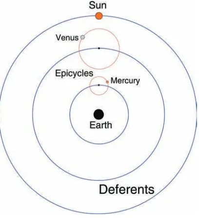
In the Ptolemaic model of the Solar System (which is more subtle than is often acknowledged), the planets move around circular ‘epicycles’ whose centres move around the Earth in larger circles, called deferents, as shown in Figure 1.2. This enables it to account for the ‘retrograde’ motion of planets like Mars and Jupiter when they appear to move backwards in the sky. It also models the motion of Mercury and Venus. In their case, the deferents, and hence the centre of their
Figure 1.1 Galileo Galilei: a portrait by Guisto Sustermans. Image: Wikipeda Commons.
Figure 1.2 The centre points of the epicycles for Mercury and Venus move round the Earth with the same angular speed as the Sun.
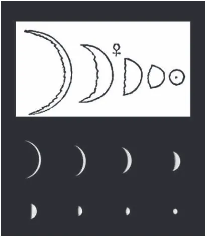
In the Ptolemaic model, Venus lies between the Earth and the Sun and hence it must always be lit from behind, so could only show crescent phases whilst its angular size would not alter greatly. In contrast, in the Copernican model Venus orbits the Sun. When on the nearside of the Sun, it would show crescent phases whilst, when on its far side but still visible, it would show almost full phases. As its distance from us would change signifi cantly, its angular size (the angle subtended by the planet as seen from the Earth) would likewise show a large change.
Figure 1.3 shows a set of drawings of Venus made by Galileo with his simple refracting telescope. They are shown in parallel with a set of modern photographs which illustrate not only that Galileo showed the phases, but that he also drew the changing angular size correctly. These drawings showed precisely what the Copernican model predicts: almost full phases when Venus is on the far side of the Sun and a small angular size coupled with thin crescent phases, having a signifi -cantly larger angular size, when it is closest to the Earth.
Galileo’s observations, made with the simplest possible astronomical instru-ment, were able to show which of the two competing models of the Solar System was correct. In just the same way, but using vastly more sophisticated instru-ments, astronomers have been able to choose between competing theories of the Universe – a story that will be told in Chapter 9.
1.3
The celestial sphere and stellar magnitudes
Looking up at the heavens on a clear night, we can imagine that the stars are located on the inside of a sphere, called the celestial sphere, whose centre is the centre of the Earth.
1.3.1 The constellations
As an aid to remembering the stars in the night sky, the ancient astronomers grouped them into constellations; representing men and women such as Orion, the Hunter, and Cassiopeia, mother of Andromeda, animals and birds such as Taurus the Bull and Cygnus the Swan and inanimate objects such as Lyra, the Lyre. There is no real signifi cance in these stellar groupings – stars are essentially seen in random locations in the sky – though some patterns of bright stars, such as the stars of the ‘Plough’ (or ‘Big Dipper’) in Ursa Major, the Great Bear, result from their birth together in a single cloud of dust and gas.
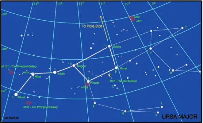
The chart in Figure 1.4 shows the brighter stars that make up the constellation of Ursa Major. The brightest stars in the constellation (linked by thicker lines) form what in the UK is called ‘The Plough’ and in the USA ‘The Big Dipper’, so called after the ladle used by farmers’ wives to give soup to the farmhands at lunchtime. On star charts the brighter stars are delineated by using larger diameter circles
which approximates to how stars appear on photographic images. The grid lines defi ne the positions of the stars on the celestial sphere as will be described below.
1.3.2 Stellar magnitudes
The early astronomers recorded the positions of the stars on the celestial sphere and their observed brightness. The fi rst known catalogue of stars was made by the Greek astronomer Hipparchos in about 130–160 BC. The stars in his catalogue were added to by Ptolomy and published in 150 AD in a famous work called the Almagest whose catalogue listed 1028 stars. Hipparchos had grouped the stars visible with the unaided eye into six magnitude groups with the brightest termed 1st magnitude and the faintest, 6th magnitude. When accurate measurements of stellar brightness were made in the nineteenth century it became apparent that, on average, the stars of a given magnitude were approximately 2.5 times brighter than those of the next fainter magnitude and that 1st magnitude stars were about 100 times brighter than the 6th magnitude stars. (The fact that each magnitude difference showed the same brightness ratio is indicative of the fact that the human eye has a logarithmic rather than linear response to light.)
In 1854, Norman Pogson at Oxford put the magnitude scale on a quantitative basis by defi ning a fi ve magnitude difference (i.e., between 1st and 6th magni-tudes) to be a brightness ratio of precisely 100. If we defi ne the brightness ratio of one magnitude difference as R, then a 5th magnitude star will be R times
brighter than a 6th magnitude star. It follows that a 4th magnitude star will be
R⫻R times brighter than a 6th magnitude star and a 1st magnitude star will be R⫻R⫻R⫻R⫻R brighter than a 6th magnitude star. However, by Pogson’s defi -nition, this must equal 100 so R must be the 5th root of 100 which is 2.512.
The brightness ratio between two stars whose apparent magnitude differs by one magnitude is 2.512.
Having defi ned the scale, it was necessary to give it a reference point. He ini-tially used Polaris as the reference star, but this was later found to be a variable star and so Vega became the reference point with its magnitude defi ned to be zero. (Today, a more complex method is used to defi ne the reference point.)
1.3.3 Apparent magnitudes
greater distance. As a result, these magnitudes are termed apparent magnitudes.
The nominal apparent magnitudes relate to the brightness as observed with instruments having the same wavelength response as the human eye. As we shall see in Chapter 6, one can also measure the apparent magnitudes as observed in specifi c wavebands, such as red or blue, and such measurements can tell us about the colour of a star.
Some stars and other celestial bodies, such as the Sun, Moon and planets are much brighter than Vega and so can have negative apparent magnitudes. Magni-tudes can also have fractional parts as, for example, Sirius which has a magnitude of ⫺1.5. Figure 1.5 gives the apparent magnitudes of a range of celestial bodies from the brightest, the Sun, to the faint dwarf planet, Pluto.
1.3.4 Magnitude calculations
From the logarithmic defi nition of the magnitude scale two formulae arise. The fi rst gives the brightness ratio, R, of two objects whose apparent
magni-tude differs by a known value ∆m:
R⫽ 2.512∆m (1.1)
The second gives the magnitude difference between two objects whose brightness ratio is known. We can derive this from the fi rst as follows:
Taking logarithms to the base 10 of both sides of Equation (1.1) gives:
Log10R⫽ Log10(2.512) ⫻∆m
Log10R⫽ 0.4 ⫻∆m
∆m⫽ Log10R/0.4
∆m⫽ 2.5 ⫻ log10R
As an example, using values from Figure 1.5, let us calculate how much brighter the Sun is than the Moon.
The difference in magnitudes is 26.7 ⫺ 12.6 ⫽ 14.1, so
R⫽ 2.51214.1
⫽ 436 800
The Sun is ∼440 000 times brighter than the full Moon.
This perhaps emphasizes the fact that the eye can cope with an incredibly wide range in brightness: we can see a surprising amount with the light of the full Moon and yet can cope with the light on a bright sunny beach.
Consider a second example: a star has a brightness which is 10 000 times less than Vega (magnitude 0). What is the magnitude of the star?
There is a quick way to do this: 10 000 is 100 ⫻ 100. However, a ratio of 100 in brightness is 5 magnitudes so this star must be 10 magnitudes fainter than Vega and will thus be 10th magnitude.
Using the formula:
∆m⫽ 2.5 ⫻ log10(10 000)
⫽ 2.5 ⫻ 4 ⫽ 10
gives the same result.
1.4
The celestial coordinate system
of the Earth and uses the orientation of the Earth in space as its basis. The Earth’s rotation axis is extended up and down to the points where it reaches our imagi-nary celestial sphere. The point where the axis meets the sphere directly above the North Pole is called the North Celestial Pole and that below the South Pole is the South Celestial Pole. If the Earth’s equator is extended outwards it will cut the celestial sphere into two – into the northern and southern hemispheres – forming the Celestial Equator (see Figure 1.6).
There is one path around the celestial sphere that is of great importance: that of our Sun. If the Earth’s rotation axis was at right angles to the plane of its orbit around the Sun, the Sun’s path would trace out the Celestial Equator but, as the axis of the Earth’s rotation is inclined to its orbital plane by an angle of 23.5°, the path of the Sun is a great circle, called the ecliptic, which is inclined by 23.5° to the Celestial Equator. The Sun spends half the year in the southern half of the celestial sphere and the other half in the northern. Its path thus crosses the Celes-tial Equator twice every year: once at the vernal equinox, on March 20 or 21, as it comes into the northern hemisphere and 6 months later when, at the autumnal equinox on September 22 or 23, it returns to the southern hemisphere.
Just as a location on the Earth’s surface has a ‘latitude’, defi ned as its angular distance from the equator towards the poles, so a star has a ‘ declination’” (Dec) given as an angle which is either positive (in the northern hemisphere) or nega-tive (in the southern hemisphere). The ‘Pole Star’ in the northern sky is close to the North Celestial Pole at close to ⫹90 declination and the region at the South
Celestial Pole (where there is no bright star) is at ⫺90 declination.
The second coordinate proves to be rather more diffi cult. On the Earth we defi ne the position of a location round the Earth by its longitude. However, there has to be some arbitrary zero of longitude. It was sensible that the zero of longitude, called the Prime Meridian, should pass through a major observatory and that honour fi nally fell to the Royal Greenwich Observatory in London.
As referred to above, the path of the Sun gives two defi ned points along the Celestial Equator that might sensibly be used as the zero of Right Ascension (RA) – the points where the ecliptic crosses the Celestial Equator at the vernal and autumnal equinoxes. The point where the Sun moves into the northern hemi-sphere was chosen and was given the name ‘The fi rst point of Aries’ as this was the constellation in which it lay. Star positions are measured eastwards around the celestial sphere from the fi rst point in Aries to give the star’s RA.
However, for reasons that will become apparent when we describe how star positions are measured, RA is not measured in degrees but in time, with 24 h equivalent to 360°. Hence, the celestial sphere is split into 24 segments each of 1 h and equivalent to 15° around the Celestial Equator.
Angular measure
A great circle measures 360° in angular extent. Each degree is divided into 60 arcmin.
Each arcminute is divided into 60 arcsec. There are then 3600 arcsec in 1°.
(Arcseconds and arcminutes can also be written as seconds of arc and minutes of arc, respectively.)
1.5
Precession
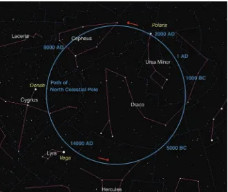
rate is slow; one rotation every ∼26 000 years, but its effect over the centuries is to change the positions of stars as measured with the co-ordinate system described above, which is fi xed to the Earth. Consequently, a star chart is only valid for one specifi c date. Current star charts show the positions of stars as they were at the start of the millennium and will state ‘Epoch 2000’ in their titles. One result of precession is that the Pole Star is only close to the North Celestial Pole at this par-ticular moment in time in the precession cycle (Figure 1.7). In ∼12 000 years, the bright star Vega will be near the North Celestial Pole instead (though by no means as close). It also means that constellations currently not observable from the UK will become visible above the southern horizon.
Interestingly, it is stars in the part of the sky that was visible to ancient astronomers and which were thus included in the constellations that enable us to estimate not only the time but also the latitude from which the constellations were delineated and named.
A region of about 36° radius in the southern sky did not contain any of the original 48 constellations implying that this region was invisible to those who
mapped the sky. This is precisely the region that would have been invisible to those living at a latitude of 36° north. Due to precession, the stars that would be hidden from view in this region will vary with time, and this enables us to give a date, about 2600–2900 BC, when the constellations were delineated. This origin would also explain the reason behind the long, thin constellation Hydra, the sea serpent, that now arcs across 95° of the sky – Hydra then followed the line of the Celestial Equator.
The ancient Greek poet, Aratus, described how some stars set as others rose into the night sky at opposite points on the horizon. Again, due to precession, such coincidences will also depend on the latitude of the observer and the time of observation. These observations also imply a latitude of about 36° north and a date about 2600 BC.
1.6
Time
Before one can appreciate the observations that lay behind a second observational triumph, which came about from the precise observations of the positions of the stars and planets by Tycho Brahe in the seventeenth century, it is necessary to understand how astronomers measure time.
1.6.1 Local solar time
For centuries, the time of day was directly linked to the Sun’s passage across the sky, with 24 h being the time between one transit of the Sun across the meridian and that on the following day. This time standard is called ‘Local Solar Time’ and is the time indicated on a sundial. The time such clocks would show would thus vary across the UK, as noon is later in the west. It is surprising the difference this makes. In total, the UK stretches 9.55° in longitude from Lowestoft in the east to Mangor Beg in County Fermanagh, Northern Ireland in the west. As 15° is equivalent to 1 h, this is a time difference of just over 38 min!
1.6.2 Greenwich mean time
As the railways progressed across the UK, this difference became an embarrass-ment and so London or ‘Greenwich’ time was applied across the whole of the UK. A further problem had become apparent as clocks became more accurate: due to the fact that the Earth’s orbit is elliptical the length of the day varies slightly. Thus, 24 h, as measured by clocks, was defi ned to be the average length of the day over
1.6.3 The equation of time
The use of GMT has the consequences that, during the year, our clocks get in and out of step with the Sun. The difference between GMT and the Local Solar Time at Greenwich is called the ‘Equation of Time’(Figure 1.8). The result is that the Sun is not always due south at noon, even in London, and the Sun can transit (cross the meridian) up to 16 min 33 s before noon as measured by a clock giving GMT and up to 14 min 6 s afterwards. This means that sunrise and sunset are not usu-ally symmetricusu-ally centred on midday and this does give a noticeable effect around Christmas time. Though the shortest day is on December 21, the Winter Solstice, the earliest sunset is around December 10 and the latest sunrise does not occur until January 2, so the mornings continue to get darker for a couple of weeks after December 21 whilst, by the beginning of January, the evenings are appreciably longer.
1.6.4 Universal time
Greenwich Mean Time was formally replaced by Universal Time (UT) in 1928 (although the title has not yet come into common usage) but was essentially the same as GMT until 1967 when the defi nition of the second was changed! Prior to this, 1 s was defi ned as 1/86 400th of a mean day as determined by the rotation of the Earth. The rotation rate of the Earth was thus our fundamental time stan-dard. The problem with this defi nition is that, due to the tidal forces of the Moon,
the Earth’s rotation rate is gradually slowing and, as a consequence, the length of time defi ned by the second was increasing. Hence, in 1967, a new defi nition of the second was made:
The second is the duration of 9 192 631 770 periods of the radiation corresponding to the transition between the two hyperfi ne levels of the ground state of the caesium 133 atom.
Thus our clocks are now related to an Atomic Time standard which uses caesium beam frequency standards to determine the length of the second.
This has not stopped the Earth’s rotation from slowing down, and so very grad-ually the synchronization between the Sun’s position in the sky and our clocks will be lost. To overcome this, when the difference between the time measured by the atomic clocks and the Sun (as determined by the Earth’s rotation rate) differs by around a second, a leap second is inserted to bring solar and atomic time back in step. This is usually done at midnight on New Year’s Eve or June 30. Since the time defi nition was changed, 22 leap seconds have had to be added, about one every 18 months, but there were none between 1998 and 2005 showing the slowdown is not particularly regular. Leap seconds are somewhat of a nuisance for systems such as the Global Positioning System (GPS) Network and there is pressure to do away with them which is, not surprisingly, opposed by astronomers! If no cor-rection was made and the average slow down over the last 39 years of 0.56 of a second per year continues, then in 1000 years UT and solar time would have drifted apart by ∼9 min.
1.6.5 Sidereal time
If one started an electronic stop watch running on UT as the star Rigel, in Orion, was seen to cross the meridian and stopped it the following night when it again crossed the meridian, it would be found to read 23 h, 56 min and 4.09 s, not 24 h. This period is called the sidereal day and is the length of the day as measured with respect to the apparent rotation of the stars.
year. In reality, during this time, the Earth has made ∼365 rotations so, in relation to the star Rigel (or any other star), the Earth has made a total of ∼365 ⫹ 1
rota-tions in 1 year and hence there are ∼366 sidereal days in 1 year. The sidereal day is thus a little shorter and is approximately 365/366 of an Earth day.
The difference would be ∼1/366 of a day or 1440/366 min giving 3.93 min or 3 min 55.8 s. The length of the sidereal day on this simplifi ed calculation is thus approximately 23 h 56 min 4.2 s, very close to the actual value.
1.6.6 An absolute time standard – cosmic time
This section is not really necessary for the development of this chapter, but the ideas described here are very interesting and allow some discussion of Einstein’s theories of relativity and the fact that, only recently, we have been able to consider how time measured by us on Earth relates to the timescale of the universe.
In 1905, Albert Einstein, then working in the Berne Patent Offi ce, published his paper on the Special Theory of Relativity. Perhaps one of the most well known aspects of this theory is that moving clocks appear to run slow when compared with a clock at rest with an observer – a phenomenon called time dilation. This prediction has been proven by fl ying highly accurate atomic clocks around the world and has to be taken into account in the GPS system used for navigation. (See the box at the end of this section.)
As time is relative can we actually defi ne a time standard with which to observe the evolution of the universe? One could, perhaps, defi ne what might be called cosmic time as that measured by a clock that is stationary with respect to the uni-verse as a whole. How would this time relate to clocks on Earth? We know that the Earth is moving around the Sun, and that the Sun is moving around the centre of our Milky Way Galaxy once every ∼220 million years. Can we measure how fast the Solar System is moving with respect to the universe? Perhaps surprisingly, we can.
about 0.22% of the speed of light). This is our speed with respect to the universe as a whole.
We can thus calculate how the time of a clock at rest with the universe – measuring cosmic time – will differ from our clocks. To do this we need to derive the formula that determines the observed time dilation as a function of relative speed. This is not diffi cult if we can imagine a very simple ‘clock’.
The clock is made by refl ecting a photon back and forth between a pair of perfect mirrors separated by a distance, d, as seen in Figure 1.9a. Our ‘tick’ happens every
time the photon refl ects off the lower mirror and so the photon will travel a distance 2d between each tick. Our fundamental time period, t1, will thus be given by:
t1⫽ 2d/c
Suppose we observe such a clock moving past us at speed v. We will see the
situa-tion in Figure 1.9b. As seen from our point of view, the photon will have to travel a longer distance, l, between each tick. This distance is given by:
l⫽ [(2d)2⫹ (vt 2)2]1/2
The time interval between each tick, t2, will then be given by:
t2⫽l/c⫽ [(4d2⫹v2t 22)/c2]1/2
(c has been squared and put inside the square root.)
Squaring both sides and cross multiplying gives;
t22c2
⫽ 4d2
⫹v2t 22
We can now relate t2 and t1 to v by substituting for d from above using d2⫽t 12c2/4, giving:
t22c2
⫽t12c2
⫹v2t 22
and
t22(c2⫺v2) ⫽t 12c2
so, fi nally,
t2/t1⫽ [c2/(c2
⫺v2)]1/2
or,
t2/t1⫽ 1/[1 ⫺ (v2/c2)]1/2
This is the time dilation formula, giving the ratio of time intervals as a function of the relative speed v.
We can now enter our speed with respect to the universe, 650 km s⫺1, into this
equation and get the ratio 1.0000023. This is exceedingly small so, to a very good approximation, our clocks can be used to measure the timescale of the universe.
Relativity and the Global Positioning System
Travelling around the globe at a speed of 3.9 km s⫺1, the atomic clocks providing the
time signals in the GPS satellite constellation will lose ∼7.2 µs day⫺1 as measured by
clocks on the ground. (You could try this calculation.) It should however be pointed out that there is an even greater effect due to the fact that the GPS clocks are in a weaker gravitational fi eld. This makes them run fast compared with clocks on the ground by 45.9 µs day⫺1. Combining the two effects gives a net offset of ⫹38.7 µs
day⫺1. To account for this, the frequency standards on board the GPS satellites are
given a rate offset prior to launch, making them run slightly slow – they are set to 10.22999999543 MHz instead of 10.23 MHz.
1.7
A second major observational triumph: the laws
of planetary motion
1.7.1 Tycho Brahe’s observations of the heavens
In 1572, Tycho Brahe, a young Danish nobleman whose passion was astronomy, observed a supernova (a very bright new star) in the constellation of Cassiopeia. His published observations of the new ‘star’ shattered the widely held belief that the heavens were immutable and he became a highly respected astronomer.
He realised that in order to show when further changes in the heavens might take place it was vital to have a fi rst class catalogue of the visible stars. Four years later, Tycho was given the Island of Hven by the King of Denmark and money to build a castle that he called Uraniborg, named after Urania, the Greek Goddess of the heavens. In the castle’s grounds, he built a semi-underground observatory called Stjerneborg. For a period of 20 years, his team of observers made positional measurements of the stars and, critically important, the planets.
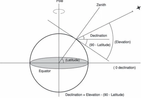
Figure 1.10b shows the observatory and Figure 1.11 indicates how the measure-ments were made. An observer sighted a star (or planet) through a small window on a south facing wall. He did two things. First, he was able to indicate to his assistants when the star crossed the meridian. (The meridian is the half-circle that runs across the sky through the zenith between the north and south poles and intersects the horizon due south.) Secondly, by using a giant quadrant equipped with vernier scales, he was able to measure the elevation (angular height above the horizon) of the star at the moment of transit. One assistant is standing beside the clock at the lower right of the diagram to measure the time at which the star transits and a second assistant is seated at a table at the lower left who would then note the elevation of the star and time of transit in the logbook. From Figure 1.12 you can see that, given its observed elevation and the latitude of the observatory, the declination of the star can be found directly.
Figure 1.11 Observing the elevation of a star as it transited due south. Observatory image: Wikipedia Commons. Note, on the original, the window is too high.
The time of the transit gives the RA. Let us now suppose that Tycho Brahe set his clock to measure sidereal time. If he now set his clock to read 0:00 h at the time when the First Point of Aries crossed the meridian, then the time when a star crossed the meridian would directly give the RA! You can now see how the convention that RA is measured in units of time and increases to the east came about.
Today, transit telescopes, such as that at the Royal Greenwich Observatory, are used to measure stellar positions. These can only observe due south and, like Tycho’s quadrant, are used to measure the elevation of a star as it transits the meridian. It is observations made by this type of telescope that have shown that, gradually, the rotation rate of the Earth has been slowing down, and they are used to decide when a ‘leap second’ should be added.
The time of transit would now be measured in UT but, given the value of the sidereal time at the previous midnight, ‘GST at midnight’ (GST is Greenwich Side-real Time), the sideSide-real time at the moment of observation, and hence the RA can be easily calculated as follows.
Suppose a star is observed to transit at 02:23:36 UT and given that the GST at the previous midnight, as found in the Nautical Almanac, was 19:16:21, a ball-park fi gure of the RA could be found by just adding these two times together to give 21:39:57. However, this simple calculation neglects to account for the fact that sidereal seconds are shorter than UT seconds, so that the increase in sidereal time since midnight will be slightly greater than the increase in UT. To the nearest second, there are (23 ⫻ 3600) ⫹ (56 ⫻ 60) ⫹ 4 ⫽ 86 164 UT seconds in 1 sidereal day. A sidereal second is thus 86 164/86 400 times shorter than a UT second (86 400 ⫽ 24 ⫻ 3600).
The accurate calculation:
The transit was 7200 ⫹ 1380 ⫹ 36 ⫽ 8616 UT seconds after midnight. This would equate to 8616 ⫻ 86 400/86 164 ⫽ 8639 sidereal seconds. This is 02:23:59 as measured in sidereal time.
The RA of the star would thus be 19:16:21 ⫹ 02:23:59 ⫽ 21:40:20. (This is 23 s greater in RA than the ball-park fi gure.)
1.7.2 Johannes Kepler joins Tycho Brahe
When King Frederik II died in 1588, Tycho lost his patron. The fi nal observation at Hven was made in 1596 before Tycho left Denmark. After a year travelling around Europe he was offered the post of Imperial Mathematician to Rudolf II, the Holy Roman Emperor, and was installed in the castle at Benatky. It was here that a young mathematician, Johannes Kepler, came to work with him. Tycho gave him the task of solving the orbit of the planet Mars. Kepler thought that it would take him a few months. In fact, it took him several years!
There was a fundamental problem. The observations of Mars had been made from the Earth, which was itself in orbit around the Sun. Unless one knew the precise orbit of the Earth, one could not fi nd the parameters of the Martian orbit. In what has been described as a stroke of genius, Kepler realized that every 687 days (the orbital period of Mars) Mars would return to exactly the same location in the Solar System, so observations of the Earth from Mars, made on a set of dates separated by 687 days, could be used to fi nd the precise orbit of the Earth. (As could, of course, observations made on those days of Mars from the Earth.) Having fi rst solved for the Earth’s orbit, Kepler was then able to deduce the orbital parameters of Mars.
1.7.3 The laws of planetary motion
From the invaluable database of planetary positions provided by Tycho, Kepler was able to draw up his three empirical laws of planetary motion. The word ‘empirical’ indicated that these laws were not based on any deeper theory, but accurately described the observed motion of the planets. The fi rst two were pub-lished in 1609 and the third in 1618.
The fi rst law states that:
Planets move in elliptical orbits around the Sun, with the Sun positioned at one focus of the ellipse.
Figure 1.13 shows a planet in an elliptical orbit around the Sun and defi nes some of the terms associated with the orbit.
The second law states that:
The radius vector – that is, the imaginary line joining the centre of the planet to the centre of the Sun – sweeps out equal areas in equal times.
Figure 1.13 The parameters of an elliptical orbit.
Figure 1.14 Kepler’s Second Law.
The third law relates the period of the planet’s orbit, T, with a, the semi-major
axis of its orbit and states that:
The square of the planet’s period,T,is proportional to the cube of the semi-major axis of its orbit,a.
One point should be made here: if an orbit is circular, then the semi-major axis is simply the radius of the circle and thus the distance of the planet from the Sun. When the orbit is not far from circular, then the semi-major axis is very close to the mean distance of the planet from the Sun. The third law is often stated in the form:
The square of the planet’s period is proportional to the cube of its mean distance from the Sun.
However, this is not strictly accurate.
It should also be noted that Kepler’s Third Law as stated above is only applicable when one of the bodies is signifi cantly more massive than the other – as is always the case for the planets of our Solar System.
Writing the third law mathematically:
T2αa3
Thus:
T2
⫽k⫻a3
where k is a constant of proportionality.
The value of k, which will be the same for all objects orbiting the Sun, depends
on the units chosen. It is conventional to measure the period, T, in units of Earth
years and the semi-major axis, a, in units of the Earth’s semi-major axis, which is
termed an Astronomical Unit (AU), in which case k⫽ 1.
The semi-major axis of the asteroid Ceres, which orbits the Sun every 4.60 years can thus be found using T2⫽k⫻a3. With k⫽ 1, this becomes a3⫽T2, and thus:
a⫽T2/3
giving a⫽ 2.77AU.
Kepler’s Third Law can, of course, be applied to any system of planets or sat-ellites orbiting a body. Only the value of the constant of proportionality will be different.
An example
satellite will orbit the Earth once per day and so remain in the same position in the sky as seen from a location on the Earth’s surface, thus allowing a fi xed reception antenna. How high above the surface of the Earth at the equator would such an orbit be?
The radius of the Moon’s orbit is 384 400 km and its orbital period is 27.32 days.
(You may be worried about this value for the period and might think that it should be 29.53 days. This latter value is the period between two New Moons, and is called the synodic lunar month. It is obviously related to the position of the Moon related to the Sun and so depends both on the Moon’s motion about the Earth and the orbital motion of the Earth–Moon system around the Sun. The
27.32 day sidereal lunar month, the value that we need to use, is determined by the time it takes for the Moon to return to the same place on the celestial sphere after one orbit of the Earth. Incidentally, Richard Feynman in his famous Feynman Lectures on Physics made this mistake and used 29.5 days as the Moon’s orbital
period – but he was a world-famous physicist, not an astronomer, so perhaps he can be forgiven!)
Using these values, we can calculate the constant of proportionality that applies to satellites around the Earth:
k⫽ (27.32)2/(384 400)3 ⫽ 1.314 ⫻ 10⫺14.
For our geostationary satellite, T is 1, so we derive “‘a’ from:
1 ⫽k⫻a3
a⫽ (1/k)1/3
⫽ 42 377 km.
The surface of the Earth is 6400 km from the centre, so geostationary satellites are ∼36 000 km above the surface of the Earth.
1.8
Measuring the astronomical unit
by the map. This would then give the scale, and thus the distance between any other two points on the map could be found.
In the case of the Solar System, the obvious measurement to make was the distance between the Earth and either of its two nearest planets, Venus or Mars. Initially this was attempted by the use of parallax: the slight difference in direc-tion of an object when viewed from different locadirec-tions. In principle, the posidirec-tion of a planet, as seen against the backdrop of the distant stars, would be different when observed from separate locations on Earth. The problem is that the widest separation possible on the Earth is approximately its diameter, 12 756 km, which is small compared with the distances of the planets. The angular difference that has to be measured is thus very small and prone to errors.
In 1672, the Italian observer Cassini observed Mars from Paris whilst a col-league observed it from French Guiana in South America (Figure 1.15). They were able to measure its parallax, and hence measure the Earth–Mars distance. Using Kepler’s Third Law they were then able to calculate the Earth’s distance from the Sun, and derived a value of 140 million km.
Later astronomers observed the transit of Venus, two of which occur each cen-tury. By timing (from locations all over the Earth) when Venus fi rst entered the Sun’s limb and then just before it left, one can measure the parallax of Venus and hence fi nd its distance. The value deduced from both the eighteenth century tran-sits was 152.4 million km (Figure 1.16).
A truly accurate measurement had to wait until 1962, when powerful radars using large radio telescopes in the USA, Russia and at Jodrell Bank in the UK, were able to obtain echoes from the surface of Venus. The accepted value now is 149 597 870.691 km, just less than 150 million km or 93 million miles.
1.9
Isaac Newton and his Universal Law of Gravity
Isaac Newton was born in the manor house of Woolsthorpe, near Grantham, in 1642, the same year Galileo died. His father, also called Isaac Newton, had died before his birth and his mother, Hannah, married the minister of a nearby church when Isaac was 2 years old. Isaac was left in the care of his grandmother and effec-tively treated as an orphan. He attended the Free Grammar School in Grantham but showed little promise in academic work and his school reports described him as ‘idle’ and ‘inattentive’. His mother later took Isaac away from school to manage her property and land, but he soon showed that he had little talent and no interest in managing an estate.
An uncle persuaded his mother that Isaac should prepare for entering university and so, in 1660, he was allowed to return to the Free Grammar School in Grantham to complete his school education. He lodged with the school’s headmaster who gave Isaac private tuition and he was able to enter Trinity College, Cambridge in 1661 as a somewhat more mature student than most of his contemporaries. He received his bachelor’s degree in April 1665 but then had to return home when the University was closed as a result of the Plague. It was there, in a period of 2 years and whilst he was still under 25, that his genius became apparent.
There is a story (which is probably apocryphal) that Newton was sitting under the apple tree in the garden of Woolsthorpe Manor. He might well have been able to see the fi rst or last quarter Moon in the sky. It is said that an apple dropped on his head (or thudded to the ground beside him) and this made him wonder why the Moon did not fall towards the Earth as well.
Newton’s moment of genius was to realise that the Moon was falling towards
the Earth! He was aware of Galileo’s work relating to the trajectories of projectiles and, in his great work Principia published in 1686, he considered what would
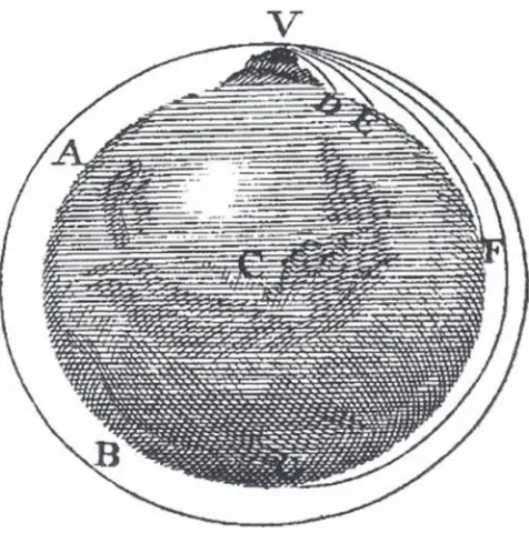
happen if one fi red a cannon ball horizontally from the top of a high mountain where air resistance could be ignored. The cannon ball would follow a parabolic path to the ground. As the cannon ball was fi red with greater and greater velocity it would land further and further away from the mountain. As the landing point becomes further away the curvature of the Earth must be considered. In a more popular work published in the 1680s called A Treatise of the System of the World,
he included Figure 1.17. The mountain is impossibly high in order for it to reach above the Earth’s atmosphere. However, this is a thought experiment, not a real one. One can see from this that, if the velocity is gradually increased there would come a point when the cannon ball would never land – and would be in an orbit around the Earth.
Let us fi rst treat this experiment quantitatively and use modern day values and units to extend Newton’s arguments to encompass the Moon. You can calculate that the surface of the Earth falls below a fl at horizontal line by approximately 5 m over a distance of 8 km. If one drops a mass from rest at the surface of the Earth, it will drop a height of ½gt2 in a time t, where g is the acceleration due to gravity at the Earth’s surface. The value of g is 9.8 m s⫺2 so the fall would be 4.9 m. So, if we fi red the cannon ball with a speed of about 8000 m s⫺1, its fall after 8 km would match the falling away of the Earth’s surface and the cannon ball would remain in orbit.
Newton applied the same logic to the motion of the Moon, realising that, if the gravitational attraction between the Earth and Moon caused it to fall by just the right amount, it too would remain in orbit around the Earth. He knew enough about the Moon to be able to calculate the value of the acceleration of gravity at the distance of the Moon. For this, he needed to know the radius of the Moon’s orbit (assumed to be circular) about the centre of the Earth, and also the period of its orbit around the Earth. Newton used a value of the radius of the Moon’s orbit of 384 000 km and a period of 27.32 days or 2.36 ⫻ 106 s. Referring to Figure 1.18 (which is not to scale) one can easily calculate the distance, L (the length AB), and
direction (tangential to the radius vector) that the Moon would travel in 1 s if sud-denly there were no gravitational attraction between the Earth and the Moon.
Using the small angle approximation, where sin θ⫽θ (in radians), then L⫽R⫻θ, so
θ⫽ (1/2.36 ⫻ 106) ⫻ 2 ⫻π⫽ 2.66 ⫻ 10⫺6 rad.
Giving L⫽ 1.022 km.
As a result of the mutual attraction of the Earth and the Moon, the Moon will actually follow the curved path AC which can be thought of as being made up of the straight line motion AB and a fall BC, the distance fallen by the Moon in 1 s.
Let the distance from the centre of the Earth, point E, to A be R and from E to B
be D. Finally let the distance from B to C be d. As the orbit is circular, the distance
from E to C is also R.
With this notation, d⫽D⫺R
In the right-angled triangle ABE, R/D⫽ cos θ, or
D⫽R/cos θ. Hence,
d⫽D⫺R⫽R/cos θ⫺R⫽R [(1/cos θ) ⫺ 1]. Now θ is a very small angle, so we may write:
cos θ⫽ 1 ⫺ (θ2/2)
where θ is in radians.
Using the binomial theorem to fi nd 1/cosθ, and ignoring all but the fi rst two terms (θ is very small) we get:
1/cos θ⫽ 1 ⫹ (θ2/2).
Substituting in the expression for BC, we obtain:
d⫽R⫻θ2/2
⫽ [3.84 ⫻ 108 m ⫻ (2.66 ⫻ 10⫺6)2] /2
⫽ 1.36 ⫻ 10⫺3 m.
Let us assume that the acceleration due to gravity at the distance of the Moon is gm, then this fall would be equal to ½gmt2 so that g
m is 0.00272 m s⫺2. This is considerably less than the value of 9.81 at the Earth’s surface, so the force of gravity must fall off as the distance between the two objects increases. The value of g at the distance of the Moon compared with that at the Earth’s
surface was 0.00272/9.81 ⫽ 2.77 ⫻ 10⫺4. This is a ratio of 1/3606. Newton knew that the radius of the Earth was 6400 km, so that the Moon, at a dis-tance of 384 000 km, was precisely 60 times further away from the centre of the Earth than the Earth’s surface. Hence, the value of g at the distance of the
Moon had fallen almost precisely by the ratio of the distances from the centre of the Earth squared!
This led Newton to his famous inverse square law: the force of gravitational attraction between two bodies decreases with increasing distance between them as the inverse of the square of that distance.
However, Newton had a problem: he felt that he could not publish his law until he could prove that the gravitational pull exerted by a spherical body was pre-cisely the same as if all the mass were concentrated at its centre. This can only be proved by calculus and it took Newton a while to develop the ideas of calculus, which he called ‘ fl uxions’. It was only then that he felt confi dent enough to pres-ent his theory to the world.
The proof is not diffi cult, but rather long: as a sphere can be regarded as set of thin nested shells, the required proof is to show that the gravitational attrac-tion of a thin shell is as if all its mass were concentrated at its geometrical centre. You will thus see that there is no requirement that the body is uniformly dense (the Earth certainly is not) but it does require that the density at a given distance from the centre is constant – the body must have a spherically symmetric mass distribution.
Newton realized that the force of gravity must also be directly proportional to the object’s mass. Also, based on his third law of motion, he knew that when the Earth exerts its gravitational force on an object, such as the Moon, that object must exert an equal and opposite force on the Earth. He thus reasoned that, due to this symmetry, the magnitude of the force of gravity must be proportional to both the masses.
His law thus stated that the force, F, between two bodies is directly proportional
to the product of their masses and inversely proportional to the distance between their centres. This can be written as:
where M1 and M2 are the masses of the two bodies and d is their separation. Thus
one can write:
F⫽G⫻M1M2/d2
which is Newton’s Universal Law of Gravitation, where G is the constant of
proportionality called the universal constant of gravitation.
Why Universal? Using his second law (force ⫽ mass ⫻ acceleration) and his Law of Gravity, Newton was able to deduce Kepler’s third law of planetary motion. This deduction showed him that his law was valid throughout the whole of the then known Solar System. To him that was Universal!
1.9.1 Derivation of Kepler’s third law
To simplify the derivation, it is assumed that the orbit of the planet is circular. The acceleration that must act on the object to keep it in a circular orbit around a body is given by:
a⫽v2/r
where v is the object’s speed in its orbit and r is the radius of the circular orbit.
Also, stating Newton’s Second Law:
F⫽m a
where F is force, m is mass and a is acceleration.
So the inward force to act on the planet to overcome its inertia and keep it in a circular orbit is:
mpv2/r.
This force is provided by the gravitational force between the Sun and the planet so:
mpv2/r
Cancelling mp and r, we get:
v2⫽Gm s/r
The period P of the orbit is simply 2πr/v, so v⫽ 2πr/P.
Thus, 4π2r2/P2
⫽Gms/r
Giving: 4π2r3
⫽G msP2
Dividing both sides by Gms and swapping sides gives:
P2⫽ (4π2/Gm s)r3.
As the part in brackets is a constant, P2 is proportional to r3 – Kepler’s Third Law! Over 300 years after the publication of his great theory, it is diffi cult to be pre-cise as to how he developed the theory in his mind. The outline above is, I am sure, how Newton would like us to believe it happened – observations leading to an inverse square law that was proven by showing that Kepler’s Third Law could be derived from it. However, it could have happened in an inverse man-ner. From Newton’s Second Law and Kepler’s Third Law one can show that the forces between the Sun and planets must follow an inverse square law. From this, Newton could calculate the value of g at the distance of the Moon, and hence
the period of its orbit by working backwards through the calculation above. This observation would then show that a prediction of the law was true. It does not really matter which was the case, Newton’s Universal Law of Gravitation was an outstanding achievement.
Newton derived a value of G by estimating the mass of the Earth assuming it
had an average density of 5400 kg m⫺3. He suspected that the Earth increases in density with increasing depth and had simply doubled the value of 2700 kg m⫺3 that is measured at the surface of the Earth. (This was a pretty good – and very lucky – estimate, as it is actually 5520 kg m⫺3!)
Again, using modern values and units, let us carry out this calculation. We derived a value for the acceleration due to gravity at the distance of the Moon, gm, above:
From Newton’s Second Law (force ⫽ mass ⫻ acceleration), the force acting on the Moon must have been:
Mm⫻ 0.00272 kg m s⫺2⫽M
m⫻ 0.00272 N
Equating this with the force between them, as calculated from his law of gravity:
G⫻MeMm/d2⫽M
m⫻ 0.00272,
Giving G⫽ 0.00272 ⫻d2/M e
(Notice that the Moon’s mass cancels out.)
With d⫽ 384 000 km ⫽ 3.84 ⫻ 108 m
and Me⫽ 5400 ⫻ 4/3 ⫻π⫻ (6.4 ⫻ 106)3 kg ⫽ 5.93 ⫻ 1024 kg
G⫽ 0.00272 ⫻ (3.84 ⫻ 108)2/5.93 ⫻ 1024 N m2 kg⫺2
⫽ 4.0 ⫻ 1014/5.93 ⫻ 1024 N m2 kg⫺2
⫽ 6.76 ⫻ 10⫺11 N m2 kg⫺2
Due to his lucky estimate of the mean density of the Earth, this was a very good result – the now accepted value of G being 6.67 ⫻ 10⫺11 N m2 kg⫺2.
1.10
Experimental measurements of G, the universal constant
of gravitation
In 1774, Nevil Maskelyne used the defl ection (about 11 arcsec) of a plumb line, on the slopes of Mt Schiehallion in Scotland, to determine the gravitational attraction between the plum bob and the mountain. He was primarily inter-ested in using this result to measure the mean density of the Earth. Schiehallion, which rises to 3547 ft (∼1081 m), has a very regular shape, and so Maskelyne was able to estimate the mountain’s mass and thus determine the value of G, but
his values for G and that of the density of the Earth (4400 kg m⫺3) were not very
accurate.
Later, in 1798, Henry Cavendish was the fi rst to measure G in the laboratory