Energy Consumption and the Size of the Informal Economy

(1)

Energy Consumption and the Size of the Informal

Economy

Mustafa Metin Basbay, Ceyhun Elgin, and Orhan Torul

Abstract

In this paper, the authors empirically investigate the relationship between energy consumption and the size of the informal economy. Relying on panel data regression models, their results show that at the aggregate level, energy intensity is inversely related to the size of the informal sector, providing actual empirical evidence on the presence of high labor and low capital intensity in the informal economy. Furthermore, the authors also find some support towards the presence of non-linearity and asymmetry in this relationship.

JEL O17 O13 P48 E26

Keywords Informal sector; energy consumption; panel data

Authors

Mustafa Metin Basbay, University of Cambridge, Department of Economics, Sidgwick

Ave, Cambridge, CB3 9DD, UK, mustafametinb@gmail.com

Ceyhun Elgin, Bogazici University, Department of Economics, Natuk Birkan Building,

34342 Bebek, Istanbul, Turkey

Orhan Torul, Bogazici University, Department of Economics, Natuk Birkan Building,

34342 Bebek, Istanbul, Turkey

Citation Mustafa Metin Basbay, Ceyhun Elgin, and Orhan Torul (2016). Energy Consumption and the Size of

(2)

1 Introduction

As it is defined by Hart (2008), informal (or shadow) economy is the collection of a set of economic activities that take place outside the framework of public and private sector bureaucratic establishments. Another definition by Ihrig and Moe (2004) defines it as a sector that produces legally produced goods and services without having to comply with government regulations.1

Informal economy is often characterized as a highly labor-intensive sector, rather than a capital-intensive one, without access to the technological frontier in production (Matthews, 1983). One explanation for this phenomenon is that the informal sector operates on a small scale in order to avoid government scrutiny. Accordingly, due to limitations on economies of scale, the informal sector pro-duces with lower capital and higher labor intensity. Another explanation for the higher labor-intensity is due to the lower operational cost of labor in the imper-fectly monitored informal sector. For instance, labor is cheaper in the informal sector than the formal sector since informal employers do not have to pay the minimum wage, severance payments or insurance premiums for their employees to the extent the formal employers do.

Since energy consumption is highly induced by capital intensity in production, considering the lower capital intensity of the informal sector, we expect that countries with larger informal sectors have lower levels of energy consumption. In this paper, we provide actual empirical evidence supporting this hypothesis that there is lower energy consumption per unit of output, in countries where the informal sector has a higher share in total production.

There is a vast empirical literature on energy consumption and its interaction with different major economic variables and indicators, e.g. with growth (Kraft and Kraft, 1978; Mahadevan and Asafu-Adjaye, 2007; Lee and Chang, 2008; Karanfil, 2008; Soytas and Sari, 2009; Payne, 2010), GDP and income (Yu and Choi, 1985; Eden and Jin, 1992; Oh and Lee, 2004; Lee, 2005; Masih and Masih, 1996). Among these papers, Karanfil (2008) deserves a special attention, as it is directly related to our paper. This paper argues that there is no significant correlation or causality between growth and energy consumption in Turkey when the presence of the informal sector is taken into account. Karanfil

1 _{See Frey and Pommerehne (1984), Loayza (1996), Johnson et al. (1997), Thomas (1999),}

(3)

(2008) further argues that this result is in strong contrast with previous studies that have obtained a positive correlation between growth and energy consumption and might be due to a negative relationship between informality and energy consumption. Moreover, in two other recent related papers Elgin and Oztunali (2014a, 2014b) show that, first for a cross-country panel and then for the Turkish economy, the relationship between several pollution indicators and the size of the informal sector is non-linear. In the former paper, they use cross-country panel data from 152 countries over the period from 1999 to 2009 and show that there is an inverse-U relationship between pollution indicators and informal sector size. In the latter paper, they obtain the same relationship using annual time-series data from the Turkish economy. As the pollution indicators are highly correlated with energy consumption, the findings of these two papers also shed light on our paper. Moreover, Biswas et al. (2012) and Mazhar and Elgin (2013) are also two related studies. In the former one, the authors argue that informal sector size is highly related to pollution levels that are one of the byproducts of energy consumption. A similar results is also obtained in the latter paper. Nevertheless, to the best of our knowledge, our paper is unique in the literature in investigating the relationship between energy consumption and informal sector size. We utilize an annual cross-country panel data set covering 159 countries over 33 year from 1980 to 2012 and we examine the relationship between the energy intensity, defined as total energy consumption as a percentage of GDP, and the size of the informal sector, similarly denoted as a percentage of GDP.

(4)

a percentage of GDP leads to less of a change in energy consumption compared to a decrease.

Our results might be particularly useful for policy-makers in shaping their attempts to construct energy policies or to combat against the informal sec-tor. Any policy tool designed to reduce informality or to forecast energy de-mand/consumption should take the negative association between informality and energy consumption into account. Furthermore, the presence of asymmetry and non-linearity should also not be overlooked when designing such policies.

The rest of the paper is organized as follows: In the next section, we shortly discuss a theoretical construct from which we obtain the empirical hypothesis we test in the subsequent sections. we introduce the data we are utilizing and the econometric methodology used for the estimations. In the third section, we provide results from our estimations in three subsections, namely linear estimations, non-linear estimations and analysis of asymmetry. Then, in section four, we provide a discussion of our results as well as present several policy implications. Finally, in the fifth section we conclude.

2 A Theoretical Discussion

In this section we shortly describe two different theoretical mechanisms on how informal sector size (as % of GDP) and energy consumption can be related to each other. To this end, we will highly utilize two different economic mechanisms provided by two papers, one by Dhawan et al. (2010) and yet another one by Elgin and Oztunali (2014a).

(5)

informal sector, would increase informal sector size and reduce formal sector size. This will limit the income capacity of the economy thereby reducing energy investment. Moreover, since the informal sector is less energy intensive, at the same time it will also reduce total energy consumption of the economy.

Yet another economic mechanism can be developed through the extension of the dynamic general equilibrium model of Elgin and Oztunali (2014a). In this model the authors construct a dynamic general equilibrium model to account for the inverted-U relationship between several pollution indicators and informal sector size as % of GDP. They model the informal sector as a highly labor intensive sector. (For the sake of simplicity they assume that the informal sector production function only employs labor but not physical capital). Elgin and Oztunali (2014a, 2014b) argue that the non-linear relationship between informality and pollution might exist due to the existence of two different channels: On the one hand, a larger (smaller) informal sector is associated with lower (higher) capital intensity and therefore less (more) pollution but, on the other hand, a larger (smaller) informal sector can also be associated with more (less) pollution simply because the informal sector does not comply with most, if not all, of the government regulations including environmental regulations and standards. Accordingly, the first channel is called the scale effect of informality and the second one is denoted as the deregulation effect. In the case of pollution, for lower levels of informality, the deregulation effect dominates the scale effect; whereas for larger levels of informality the opposite is true. One can extend the same reasoning to energy consumption rather than pollution and argue that these two effects also exist in this context as well. Specifically, the deregulation effect in this case implies that a larger informal economy should be associated with a higher level of energy consumption as the energy consumers in the informal economy might tend to overuse energy as they operate in the shadows.2 On the other hand, the scale effect implies that the informal sector size and energy consumption are negatively related to each other. This is again due to the fact that the capital use intensity3is

2 _{Notice that the Kaufman–Kaliberda approach to estimate the size of the informal economy is}

entirely based on the assumption that the informal economy illegally overuses electricity.

3 _{Surely, the concept of economies of scale relates to the characteristics of the technology that}

(6)

lower in the informal sector which limits the energy consumption. Depending on the relative strengths of these two effects, one can obtain a positive or negative relationship between energy consumption and informal sector size as % of GDP.

3 Data and Methodology

3.1 Data

Although the literature on the informal sector and its interaction with economic variables is ever growing, one of the major challenges in documenting rigorous and consistent empirical results is due to the difficulties in the measurement of the actual size of informality. Majority of the earlier studies in the literature try to infer the size of informality by relying on country or region-specific design, thereby lacking consistency and comparability in their construction. Schneider et al. (2010), and Schneider (2005) being the exceptions, employ the Multiple Indicators Multiple Causes (MIMIC) methodology to predict the size of infor-mality, yet offer measures only for a limited window of time. Elgin and Oztunali (2012) introduce a model-based approach to the literature by inferring the size of informality from a two-sector dynamic general equilibrium model. By doing so, they offer a new panel data set on the size of the informal economy for a large set of countries. Contrary to the earlier literature, they build on microeconomic foundations in their calibration technique, and do not rely onad-hoceconometric specifications in measuring the size of informality, hence succeed in limiting hazards in measurement error.4

In this study, we utilize the annual cross-country informal sector estimates (measured as a share of the formal economy) by Elgin and Oztunali (2012) for a

of using more capital in the informal sector relative to the formal sector such as possibly lower costs related to maintenance and equipment warranty. Nevertheless, micro-level studies on informality using firm-level data generally indicate that the capital intensity in the informal sector is much lower than in the formal sector.

4 _{To the best of our knowledge, the data set by Elgin and Oztunali (2012) offers the longest-horizon}

(7)

Table 1:Descriptive Statistics for the Full Sample

Variables Obs. Mean Std.Dev. Min Max

Informal Sector Size (IS)5 5001 0.3356 0.1375 0.0797 1.1338 Energy Intensity (EI)6 4679 0.0144 0.0162 0.0000 0.1906

panel of 159 countries between the years 1980 and 2012. We should also notice that these estimates are obtained on the assumption that the formal GDP does not include informal value-added. To proxy for measuring energy intensity, we use data provided by the U.S. Energy Information Administration (EIA) on annual energy consumption in million kilowatt hours as a percentage of GDP for the same 159 countries and sample period. Contrary to the informal sector data series, energy consumption series includes total energy consumption within an economy originating from both formal and informal sectors. Descriptive statistics of the variables of interest are displayed in Table 1.

As displayed in Table 1, the size of the informal sector is approximately one-third of real output in our data set, and its variation is considerable across countries: the standard deviation is more than one third of the mean value. While developed countries tend to have smaller sizes of the informal sector (as low as 7.97% for Switzerland in 2012), developing countries are observed to have very large informal sector sizes: in some instances, sizes even greater than 100% of their formal output. Energy intensity variable suggests approximately 14,400 thousand kilowatts of energy per unit of output is consumed in our panel data set, and the standard deviation of energy consumption per unit of output is above 100% of its mean value.

In order to investigate the relationship between energy intensity and the size of the informal sector in depth, we make use of 5 different mutually-inclusive categories, namelyoil-importing economies, emerging economies, G20, G27, and OECD. By doing so, we factor in differences due to different governmental

5 _{As discussed, informal sector size is measured as a share of the formal sector (GDP) size, which}

is why theIStakes values higher than 100% in some cases, such as in Equatorial Guinea between 1982 and 1991.

6 _{We generate the energy intensity index as energy consumption in million kilowatts divided}

(8)

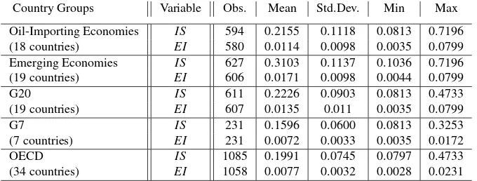
Table 2:Descriptive Statistics, Country Groups

Country Groups Variable Obs. Mean Std.Dev. Min Max

Oil-Importing Economies IS 594 0.2155 0.1118 0.0813 0.7196

(18 countries) EI 580 0.0114 0.0098 0.0035 0.0799

Emerging Economies IS 627 0.3103 0.1137 0.1036 0.7196

(19 countries) EI 606 0.0171 0.0098 0.0044 0.0799

G20 IS 611 0.2226 0.0903 0.0813 0.4733

(19 countries) EI 607 0.0135 0.011 0.0035 0.0799

G7 IS 231 0.1596 0.0600 0.0813 0.3253

(7 countries) EI 231 0.0072 0.0033 0.0035 0.0172

OECD IS 1085 0.1991 0.0745 0.0797 0.4733

(34 countries) EI 1058 0.0077 0.0032 0.0028 0.0231

ISandEIstand for informal sector size and energy intensity, respectively.

regulations, institutions, and revenue-raising activities. Further, category-specific findings enhance the robustness of our estimations, along with grasping hetero-geneity among country groups in terms of the energy intensity and informal sector size relationship.7 Descriptive statistics of variables of interest for different country groups8are illustrated in Table 2.

In addition to the aforementioned groups, we also categorize countries in five sub-groups according to their average informal sector sizes. This analysis allows us address and condition possible heterogeneities in the relationship of interest

vis-`

a-visthe informal sector size. Descriptive statistics for different country groups categorized with respect to their average informal sector sizes is provided in Table 3.

Table 3 demonstrates that both energy intensity and the informal sector size varies considerably in first and second moments among sub-groups once countries once they are conditioned on the informal sector size.

By employing the described data set, we next turn to econometrical methods to explore the nature of the informal sector and energy intensity relationship.

7 _{In Section 3, we show that the significant negative relationship between the size of the informal}

sector and energy intensity is common to all country groups, even though with different elasticities, whereas the non-linearity and asymmetric nature of this relationship may not apply to all country groups.

(9)

Table 3:Descriptive Statistics, Country Groups according to the informal sector (IS) Size

Country Groups Variable Obs. Mean Std.Dev. Min Max

IS>0.5 IS 469 0.5831 0.1194 0.2525 1.1338

(15 countries) EI 412 0.0149 0.0185 0.0004 0.1460

0.4–0.5 IS 946 0.4472 0.0489 0.3033 0.5746

(31 countries) EI 908 0.0138 0.0163 0.0018 0.1075

0.3–0.4 IS 1767 0.3510 0.0456 0.2096 0.5160

(56 countries) EI 1625 0.0164 0.0201 0.0011 0.1906

0.2–0.3 IS 701 0.2636 0.0337 0.1740 0.3919

(22 countries) EI 663 0.0114 0.0064 0.0000 0.0334

<0.2 IS 1118 0.1581 0.0351 0.0797 0.2567

(35 countries) EI 1071 0.0133 0.0120 0.0014 0.0799

3.2 Econometric Specifications

In our econometric specifications, we rely on panel-data techniques put forward by Baltagi and Wu (1999). Although our data set is quite balanced in terms of the country-year observations, there are still some absent data points in our data set. Similar to Baltagi and Wu (1999), we address this issue by employing unequally-spaced cross-sectional time-series data regression models. Further, when the disturbance term is first-order autoregressive of order one, AR(1), the proposed method is applicable, and we apply this suitable technique in our estimations, as we detect first-order autoregressive persistence in the error terms by the use of the Wooldridge test.9

Linear Specification

We start our econometric hypothesis testing for the presence of a negative relation-ship between the size of the informal sector and energy intensity by employing a log-linear ordinary least squares (OLS) estimation. The baseline estimation can

9 _{As a robustness check and to capture persistence, potentially mean-reverting dynamics as well as}

(10)

be described as follows:

log(EIi,t) =αi+β0+β1log(ISi,t−1) +β2log(EIi,t−1) +β3t+εi,t (1)

whereEIi,t stands for the energy intensity for the countryifor yeart. Similarly, ISi,t−1 stands for the size of the informal sector for countryifor the yeart−1. We also control for the time-trend through to account for the global evolution of the size of the informal sector over time. In our estimations, we also include a country-fixed dummy variables to capture region-specific peculiarities.10,11

The Wooldridge test rejects the absence of autocorrelation for the error term,

εi,t, accordingly we specify the error term to follow the below stochastic process:

εi,t=ρ+εi,t−1+zi,t (2)

where|ρ|<1 and zi,t are independent and identically distributed (i.i.d.) with

mean 0 and varianceσ2 z.

We use lagged values of the size of the informal sector so that the timing of the events could be interpreted as a causation between informality and energy intensity, i.e. the size of informality predicts energy intensity due to the timing of events, but not the other way around.12

While taking first-order difference induces loss of information, in order to check for the robustness of our findings, we also make use of regressions from first-order log differences. The first-order differences of the variables of interest can be interpreted as their annual growth rates in percentage terms.13 The model

10_{While we base our discussion through our findings from the log-linear specification, our findings}

from estimations in levels provide similar results. For brevity, we refrain from reporting these results, and they are available upon request.

11_{In our econometric specification, we employ a bivariate model to investigate the relationship}

between energy intensity and the informal sector size. Accordingly, a valid concern about our results might be associated with omitted variable bias, particularly about factors that might be associated with the magnitudes of both of the variables, such as the quality of institutions or degree of rule of law in act. The main issue about extending a bivariate model is that these variables do not tend to have high variation within a country over time, therefore could promote multicollinearity problems linked with country-specific dummy variables. To address these concerns, instead of introducing a regressor, we also cluster countries with similar economic foundations, as in the G7 group or countries with an informal sector size within the 20%-30% interval so minimize omitted variable bias.

12_{When we rely on contemporaneous timing for the informal sector variable, we derive similar}

results. These findings are available from the corresponding author upon request.

13_{Taking first differences also addresses issues considering the stationarity problems of I(1) series.}

(11)

with the first-order logarithmic differences can be expressed as follows:

∆log(EIi,t) =αi+β0+β1∆log(ISi,t−1) +β2∆log(EIi,t−1) +β3t+εi,t (3)

We use both level and first-difference specifications to investigate the rela-tionship in different country groups, as well. First, we analyze the relarela-tionship within different country groups, such as OECD, G20, G7, emerging economy or oil-importing countries; then, we repeat the same exercise also for countries categorized in terms of their average informal sector sizes. This approach pro-vides us with information about the robustness of the relationship in countries with different characteristics, especially in terms of rule of law, regulations and resources. Further, it helps us show if there are differences across countries in terms of power and significance of the relationship.

Non-Linear Specification

Our findings from both level and first-difference regressions suggest different coefficients for countries with different average sizes of informality over the years. Accordingly, we consider the possibility of a non-linear relationship between the variables of our interest. For this goal, we run the following panel-data regression:

EIi,t=αi+β0+β1ISi,t−1+β2IS2i,t−1+β3EIi,t−1+β4t+εi,t (4)

In this estimation, wheneverβ2is significantly different from zero, the rela-tionship to our interest suggests non-linearities, and depending on the magnitudes of theβ1and theβ2coefficients, convexities or concavities could arise.

Asymmetric Specification

(12)

log(EIi,t) =αi+β0+β1log(ISi,t−1) +β2log(ISi,t−1)×Dt−1 +β3log(EIi,t−1) +β4t+εi,t

(5)

whereDt−1refers to a dummy variable taking the value of 1 when the size of the informal sector increases in periodt−1, and zero otherwise.

Using this specification, we can detect if the linear relationship between the size of the informal sector and energy intensity displays asymmetry with respect to the direction of change in the size of the informal sector by focusing on theβ2 coefficient.

4 Results

4.1 Estimation Results with Linear Specification

In this section, we start by reporting our results from the benchmark linear specification.

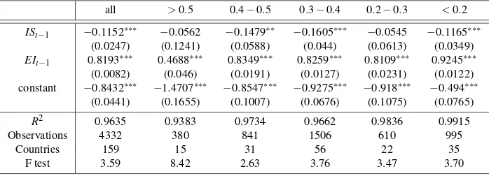
Table 4 displays the results from the level regressions employing the informal size and energy intensity variables, both expressed in their natural logarithms. In line with our expectations, we detect a negative and statistically significant relationship between the informal sector size and the energy intensity variables. The coefficient attached to the lagged informal sector size variable is significant for the whole data-set, as well as for all country sub-groups, except for the G7, which is a group of industrialized democracies (France, Germany, Italy, the United Kingdom, Japan, the United States, and Canada) with limited informal sector size and variability in informality. Notice that we run two regressions using the whole dataset one with informal sector and energy intensity and yet another one with GDP per-capita among independent variables to see whether another variable, like the natural logarithm of GDP per-capita (obtained from the Penn World Tables 8.1), plays a role in this relationship. However, it turns out that the estimated coefficient of GDP per-capita is not significant. This might be due to the fact that the already controlled lagged informal sector size and energy use intensity variables capture the variation coming from the variation in GDP per-capita.14

14_{We also have experimented some regressions with growth rate of GDP as well as some}

(13)

Table 4:Level Analysis; Country Groups

All All Oil-Importing Emerging G 20 G 7 OECD

ISt−1 −0.1152∗∗∗ ₋₀_.₁₁₅₄∗∗∗ ₋₀_.₀₆₆₀∗∗ ₋₀_.₁₃₄₁∗∗∗ ₋₀_.₀₅₀₃∗ ₋₀_.₁₃₆₄ ₋₀_.₀₇₇₈∗∗

(0.0247) (0.0245) (0.0264) (0.0265) (0.0294) (0.0864) (0.0327)

EIt−1 0.8193∗∗∗ 0.8322∗∗∗ 0.9513∗∗∗ 0.9579∗∗∗ 0.9141∗∗∗ 0.9586∗∗∗ 0.9177∗∗∗ (0.0082) (0.0081) (0.0108) (0.0137) (0.0147) (0.0213) (0.0105) constant −0.8432∗∗∗ −0.8398∗∗∗ −0.3276∗∗∗ −0.2825∗∗∗ −0.3549∗∗∗ −0.4527∗∗∗ −0.5016∗∗∗

(0.0441) (0.0439) (0.0605) (0.0624) (0.0623) (0.1599) (0.0755) GDP per-capitat−1 0.001

(0.002)

R2 _0.9635 _0.9659 _0.9793 _0.9809 _0.9941 _0.9827 _0.9799 Observations 4332 4332 544 568 563 217 990

Countries 159 159 18 19 19 7 34

F-test 3.59 3.30 4.92 4.36 3.53 2.77 4.49

Noticeably, there is considerable variation in the immediate response of energy intensity to a change in the size of the informal sector. For instance, while a 1% increase in the size of the informal sector generates approximately a 0.13% immediate decrease in energy intensity in the emerging countries on average, the correspondent decrease for the G20 country group is as low as 5%.

In Table 5, we report the results of the same econometric specification for country groups categorized in terms of their average informal sector sizes. The relationship is robust to different average informal sector sizes except for with limited country sizes, e.g. the country group with informal sector size greater than 50% of formal output, in which there are only 15 countries and issues considering non-linearity of the relationship is possible, which is addressed in the following estimations.

Table 5:Level Analysis; Countries with different average informal sector sizes

all >0.5 0.4−0.5 0.3−0.4 0.2−0.3 <0.2

ISt−1 −0.1152∗∗∗ −0.0562 −0.1479∗∗ −0.1605∗∗∗ −0.0545 −0.1165∗∗∗

(0.0247) (0.1241) (0.0588) (0.044) (0.0613) (0.0349)

EIt−1 0.8193∗∗∗ 0.4688∗∗∗ 0.8349∗∗∗ 0.8259∗∗∗ 0.8109∗∗∗ 0.9245∗∗∗

(0.0082) (0.046) (0.0191) (0.0127) (0.0231) (0.0122)

constant −0.8432∗∗∗ −1.4707∗∗∗ −0.8547∗∗∗ −0.9275∗∗∗ −0.918∗∗∗ −0.494∗∗∗

(0.0441) (0.1655) (0.1007) (0.0676) (0.1075) (0.0765)

R2 0.9635 0.9383 0.9734 0.9662 0.9836 0.9915

Observations 4332 380 841 1506 610 995

Countries 159 15 31 56 22 35

F test 3.59 8.42 2.63 3.76 3.47 3.70

(14)

Table 6:Log Differences; Country Groups

all oil-importing emerging G 20 G 7 OECD

∆ISt−1 −0.4777∗∗ −0.5865∗∗ −0.4066 −0.3111∗∗ −1.017∗∗ −0.8043∗∗ (0.1696) (0.2551) (0.2630) (0.0403) (0.4206) (0.2097)

∆EIt−1 −0.1636∗∗ −0.2331∗∗ −0.2317∗∗ −0.3111∗∗ −0.1795∗∗ −0.2961∗∗ (0.0151) (0.0433) (0.0415) (0.0403) (0.0678) (0.0302) constant 0.0094∗ −0.0123∗∗ 0.0225∗∗ −0.0055 −0.0136 −0.0084∗∗

(0.0048) (0.0038) (0.0052) (0.0039) (0.0042) (0.0029)

R2 0.2970 0.4556 0.4621 0.3437 0.3593 0.5004

Observations 4173 526 549 544 210 956

Countries 159 18 19 19 7 34

F test 1.11 4.93 2.94 3.60 3.25 2.66

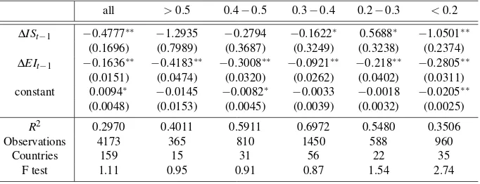
Table 7:Log Differences; Countries with different average informal sector sizes

all >0.5 0.4−0.5 0.3−0.4 0.2−0.3 <0.2

∆ISt−1 −0.4777∗∗ −1.2935 −0.2794 −0.1622∗ 0.5688∗ −1.0501∗∗ (0.1696) (0.7989) (0.3687) (0.3249) (0.3238) (0.2374)

∆EIt−1 −0.1636∗∗ −0.4183∗∗ −0.3008∗∗ −0.0921∗∗ −0.218∗∗ −0.2805∗∗ (0.0151) (0.0474) (0.0320) (0.0262) (0.0402) (0.0311) constant 0.0094∗ −0.0145 −0.0082∗ −0.0033 −0.0018 −0.0205∗∗

(0.0048) (0.0153) (0.0045) (0.0039) (0.0032) (0.0025)

R2 0.2970 0.4011 0.5911 0.6972 0.5480 0.3506

Observations 4173 365 810 1450 588 960

Countries 159 15 31 56 22 35

F test 1.11 0.95 0.91 0.87 1.54 2.74

While highR2values indicate possible problems in stationarity of the variables in use, our results from the first-difference regressions, which we illustrate in Table 6 and Table 7 provide similar qualitative findings.

(15)

and first-order estimations yield reasonableR2values, alleviating concerns on the unit-root problem in the variables of interest.

In Table 7, we condition countries with respect to their average informal sector sizes as we do in Table 5, and repeat our estimations by utilizing the logarithmic first differences instead of using logarithmic levels. The negative relationship is significant for 3 groups of countries which have average informal sector sizes as a share of formal GDP between 30% & 40%, 20% & 30% and lower than 20%. Negative relationship does not show up to be significant for countries with informal sector size higher than 50% and between 40% & 50%, again possibly due to considerable heterogeneity in these developing economies with substantial variations over time, thereby magnifying standard errors. Overall, these estimations promote the conclusion that the negative relationship is robust for country groups with different average informal sector sizes below 40% as a share of formal GDP.

Next, in order to check potential non-linearities, we turn to testing for quadratic implications of informality on the convexity and/or concavity on the relationship of our interest.

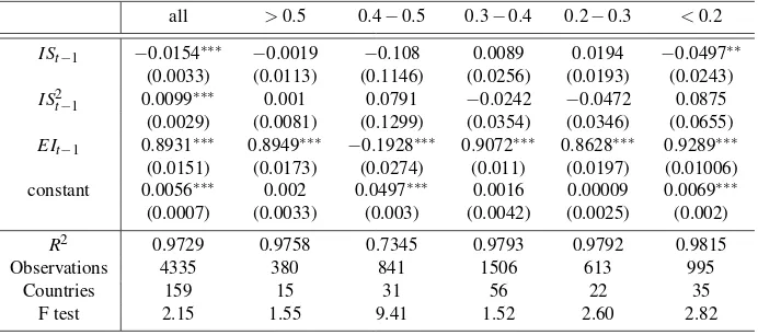
4.2 Non-Linear Estimation

In Table 8 and Table 9, we report our results from the non-linear specifications described in Equation (4). Estimated coefficients are significant only over all countries in the data; but, significant for sub-groups of countries. We interpret this findings as that sufficient number of observations, and accordingly variation is a necessary condition to detect a statistically significant non-linearity in the relationship between energy intensity and informality.

When we focus on the estimation results from the whole sample, the sig-nificant coefficients of the informal sector size,β2, and square of the informal sector size,β3are negative and positive, respectively. This finding indicates a U-shaped non-linear relationship between informality and energy intensity over all set of countries. For moderately low and very high levels of informal sector size, we detect high levels of energy intensity, whereas medium levels of informality corresponds to lower levels of energy intensity.

(16)

Table 8:Non-linear Estimation; Country groups

all oil-importing emerging G 20 G 7 OECD

ISt−1 −0.0154∗∗∗ 0.0052 −0.0064 −0.0105 −.0027 −0.0022

(0.0033) (0.0038) (0.004) (0.0081) (0.0098) (0.0044)

IS2

t−1 0.0099∗∗∗ −0.0083∗∗ 0.0011 0.0085 −0.0007 0.0010

(0.0029) (0.0037) (0.0042) (0.0118) (0.0139) (0.0062)

EIt−1 0.8931∗∗∗ 0.9204∗∗∗ 0.9273∗∗∗ 0.9353∗∗∗ 0.9499∗∗∗ 0.9223∗∗∗

(0.0151) (0.0073) (0.0091) (0.0097) (0.0241) (0.0096) constant 0.0056∗∗∗ 0.00016 0.0035∗∗∗ 0.0029∗∗∗ 0.0008 0.001

(0.0007) (0.0006) (0.0008) (0.0011) (0.0009) (0.0006)

R2 _0.9729 _0.9953 _0.9866 _0.9911 _0.9937 _0.9843

Observations 4335 544 568 563 217 990

Countries 159 18 19 19 7 34

F test 2.15 6.69 8.93 4.61 1.26 4.31

Table 9:Non-linear Estimation; Countries with different informal sector sizes

all >0.5 0.4−0.5 0.3−0.4 0.2−0.3 <0.2

ISt−1 −0.0154∗∗∗ −0.0019 −0.108 0.0089 0.0194 −0.0497∗∗

(0.0033) (0.0113) (0.1146) (0.0256) (0.0193) (0.0243)

IS_t2₋₁ 0.0099∗∗∗ 0.001 0.0791 −0.0242 −0.0472 0.0875

(0.0029) (0.0081) (0.1299) (0.0354) (0.0346) (0.0655)

EIt−1 0.8931∗∗∗ 0.8949∗∗∗ −0.1928∗∗∗ 0.9072∗∗∗ 0.8628∗∗∗ 0.9289∗∗∗

(0.0151) (0.0173) (0.0274) (0.011) (0.0197) (0.01006) constant 0.0056∗∗∗ 0.002 0.0497∗∗∗ 0.0016 0.00009 0.0069∗∗∗

(0.0007) (0.0033) (0.003) (0.0042) (0.0025) (0.002)

R2 0.9729 0.9758 0.7345 0.9793 0.9792 0.9815

Observations 4335 380 841 1506 613 995

Countries 159 15 31 56 22 35

F test 2.15 1.55 9.41 1.52 2.60 2.82

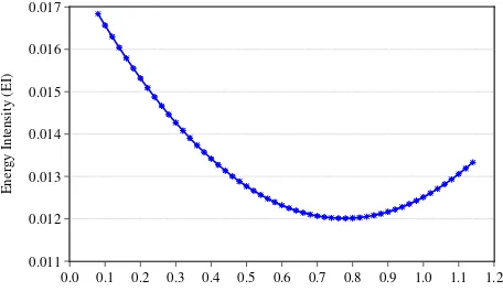
a decreasing rate and starts to increase with an increasing rate beyond a large threshold informal sector size of approximately 80%. As the size of the informal economy reaches 80%, further increases in the informal sector size actually amplifies energy intensity.

(17)

Figure 1:Non-Linear Response of Energy Intensity to Informal Sector Size

of informal sector size leads to lower levels of energy usage, which is the main mechanism through which informality affects energy intensity. Because the informal sector has to operate on a small scale to avoid being inspected by the regulatory agencies, the informal sector tends to operate by relying less on capital and more on labor. As labor intensity typically coincides with lower levels of energy usage, an increase in the informal sector size is likely to lead to a lower level of energy intensity.

(18)

Next, we turn to investigating whether an increase and decrease of equal magnitude in informal sector size induces comparable reverse quantitative impli-cations on energy intensity.

4.3 Analysis of Asymmetry

In this subsection, we present our results from the econometric specification (as described in Equation 5) to detect possible asymmetries in the relationship between the size of the informal economy and energy intensity.

In Table 10, we report that for the whole sample the negative linear rela-tionship between the size of the informal sector is robust and significant, and is not significantly asymmetric (vis-a-vis` the sign of the change in the informal sector size) at the aggregate level. Further, our estimations reveal no significant asymmetry in the relationship of interest for country subgroups except for the G20 category. The relationship for the G20 group, however, suggests that energy intensity reacts differently to an upward versus a downward change in the size of informality. Asβ2 is significantly greater than zero, we report that energy intensity responds less in magnitude to an increase in the informal sector size compared to a decrease of equal magnitude.15

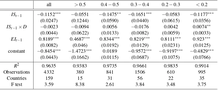
In Table 11, we report the results of the same regression for country groups conditioned in terms of average size of the informal sector. The coefficient before the dummy variable is positive, and statistically significant only for the country group with average informal sector size below 20%. It is also worth-mentioning that out of the 35 countries, only 9 out of 19 the G20 countries fall into this category.

Overall, one can conclude that for developed countries with limited informal-ity, the negative relationship between the size of the informal sector and energy intensity displays asymmetry, and suggests that a decrease in the informal sector size generates a higher impact compared to an increase of equal amount.

15_Since_D

t takes a value of 1 andβ2>0, when the size of the informal sector increases, our

(19)

Table 10:Analysis of Asymmetry; Country Groups

All Sample oil-importing emerging G 20 G 7 OECD

ISt−1 −0.1152∗∗∗ −0.0674∗∗ −0.1379∗∗∗ −0.06∗∗ −0.1061 −0.0794∗∗

(0.0247) (0.0263) (0.0268) (0.0302) (0.0815) (0.0331)

ISt−1×D −0.0023 0.0024 0.0064 0.0126∗∗∗ 0.0115∗∗ 0.0029

(0.0044) (0.00402) (0.0047) (0.0038) (0.0045) (0.0026)

EIt−1 0.8189∗∗∗ 0.9521∗∗∗ 0.9602∗∗∗ 0.9128∗∗∗ 0.9635∗∗∗ 0.917∗∗∗

(0.0082) (0.0107) (0.0139) (0.015) (0.0199) (0.0107)

constant −0.8454∗∗∗ −0.3256∗∗∗ −0.2738∗∗∗ −0.3531∗∗∗ −0.377∗∗ −0.4952∗∗∗

(0.0443) (0.0605) (0.0627) (0.0621) (0.1593) (0.0756)

R2 0.9635 0.9925 0.9806 0.9933 0.9881 0.9795

Observations 4332 544 568 563 217 990

Countries 159 18 19 19 7 34

F test 3.59 4.96 4.42 3.79 2.65 4.42

Table 11:Analysis of Asymmetry; Countries with different average informal sector sizes

all >0.5 0.4−0.5 0.3−0.4 0.2−0.3 <0.2

ISt−1 −0.1152∗∗∗ −0.0551 −0.1475∗∗ −0.1651∗∗∗ −0.0583 −0.1177∗∗∗

(0.0247) (0.1244) (0.0590) (0.0440) (0.0615) (0.0356)

ISt−1×D −0.0023 −0.0094 0.0056 −0.0176 0.0042 0.0074∗∗

(0.0044) (0.0622) (0.0133) (0.0082) (0.0059) (0.0033)

EIt−1 0.8189∗∗∗ 0.4687∗∗∗ 0.8344∗∗∗ 0.8219∗∗∗ 0.8111∗∗∗ 0.923∗∗∗

(0.0082) (0.046) (0.0192) (0.0129) (0.0231) (0.0125)

constant −0.8454∗∗∗ −1.4723∗∗∗ 0.0189 −0.9572∗∗∗ −0.9197∗∗∗ −0.4829∗∗∗

(0.0443) (0.1662) (0.0115) (0.0687) (0.1075) (0.0766)

R2 0.9635 0.9383 0.9735 0.9661 0.9835 0.9914

Observations 4332 380 841 1506 610 995

Countries 159 15 31 56 22 35

F test 3.59 8.38 2.61 3.84 3.48 3.75

5 Discussion of Results

As we have discussed in previous sections, we have three main findings in our empirical analysis:

(20)

with respect to different sets of countries. Considering the fact that the informal sector, as opposed to the formal sector, is generally characterized as a highly labor-intensive sector (but not capital intensive), we believe that this result is not surprising, yet is critical to provide actual evidence to support consequential theoretical modeling.

Second, we also document that there is a non-linear relationship between informality and energy intensity. Low and high levels of informality correspond to higher levels of energy intensity whereas medium levels of informality corre-sponds to lower levels of energy intensity. However, the bottom U-relationship is estimated to be at very high levels of informality (80 % of GDP), which means that the negative relationship between informality and energy consumption also survives the check for non-linearity. As also explained thoroughly in the second section of our paper, for a similar relationship between informality and pollution indicators Elgin and Oztunali (2014a, 2014b) argue that the non-linear relation-ship between informality and pollution might exist due to the existence of two different channels: Scale and deregulation effects of informality. In this paper, we do not provide actual empirical evidence in favour of the existence of these two forces in our context; however overall, these two mechanisms working in opposite directions might be the underlying causes behind the non-linearity we documented in our analysis. However, in our case, even though we observe some non-linearity in our regressions (at least for the whole dataset), the scale effect is much stronger; which is the main reason behind the dominating negative relationship between energy consumption and informal sector size.

Finally, we also show that there is an asymmetric relationship between infor-mality and energy consumption for a group of countries. Our results suggest that energy consumption reacts less to an increase in informal sector size compared to an decrease so that a decrease in energy consumption boosts energy consumption as a percentage of GDP. This particular feature of the relationship between energy consumption and informality is true for countries with informal sector size lower than 20% of GDP and G20 countries.

(21)

con-sumption and if the energy supply is limited in the short-run, this can cause other problems when a government is trying to reduce informal sector size.

Similarly, policy makers that are concerned about energy consumption within an economy should also be concerned about the presence of the informal sector as well as its relationship with energy consumption. Specifically, the three main findings we outlined above also shed light on the design of energy policies. First, energy policy designers should take the negative association between informality and energy consumption into account, as varying informality might have profound effects on energy demand, as well as in energy prices. Particularly, our findings suggest that policies designed to reduce informality are likely to have a positive impact on energy demand, and accordingly this can create energy shortages or considerable increases in energy prices when supply is limited. Thus, countries that are combatting against the informal sector should take appropriate precau-tionary measures in energy infrastructure and energy policy design to fine-tune the energy demand.

Second, our results with respect to the non-linearity of the relationship imply that the elasticity of energy consumption with respect to the informal sector size changes with varying informality; which should not be overlooked when constructing energy policies. That is, decreasing and increasing informal sector size are not associated with the same level of a change in energy consumption. This result is particularly important in the development path of an economy when informal sector size experiences a transition from large to smaller levels. In other words, the energy policy designed to tackle the increasing energy demand as a result of decreasing the informal sector at a certain sector size is not likely to work again properly once the informal sector size changes.

Finally, for countries with smaller informal sector size, the asymmetric nature of the relationship should also be taken into account. That is, the effect of a reduction in informal sector size has a larger effect on energy demand compared to an increase. Therefore, policy makers of these countries should also design similarly asymmetric responses for energy policy.

6 Conclusion

(22)

variables. Moreover, we also obtain some evidence for the presence of non-linearity and asymmetry in this relationship.

We should indicate that our empirical findings are highly aggregate and a deeper empirical investigation is needed, especially at the microeconomic (firm or household) level. Moreover, a further analysis is also required on the theoretical side to understand the economic mechanism behind our empirical observations. A full-fledged theoretical model incorporating energy consumption as well as informality can be constructed to gain a deeper insight of our empirical analysis. These we leave for future research.

Acknowledgements: We would like to thank the faculty at the Department of

(23)

References

[1] Arellano M., Bond, S.R. (1991). Some specification tests for panel data: Monte Carlo evidence and an application to employment equations.Review of Economic Studies, 58 (2), 277–298.

http://restud.oxfordjournals.org/content/58/2/277.short

[2] Baltagi, B.H., Wu, P.X. (1999). Unequally spaced panel data regressions with AR (1) disturbances.Econometric Theory, 15 (6), 814–823.

https://ideas.repec.org/a/cup/etheor/v15y1999i06p814-82315.html

[3] Biswas, A.K, Farzanegan, M. R., Thum, M. (2012). Pollution, shadow economy and corruption: Theory and evidence.Ecological Economics, 75,114–125.

http://www.sciencedirect.com/science/article/pii/S0921800912000092

[4] Dhawan, R., Jeske, K., Silos, P. (2010). Productivity, energy prices and the great moderation: A new link.Review of Economic Dynamics, 13(3), 715–724.

[5] Eden, S.H., Jin, J.C. (1992). Cointegration tests of energy consumption, income, and employment.Resources and Energy, 14 (3), 259–266.

http://www.sciencedirect.com/science/article/pii/016505729290010E

[6] Elgin, C., Oztunali, O. (2012). Shadow Economies all around the world: Model based estimates. Bogazici University Economics Department Working Pa-pers, 2012–05.

https://ideas.repec.org/p/bou/wpaper/2012-05.html

[7] Elgin, C., Oztunali, O. (2014a). Pollution and informal economy.Economic Systems, 38(3), 333–349.

[8] Elgin, C.,Oztunali, O. (2014b). Environmental Kuznets curve for the informal sector of Turkey: 1950-2009.Panoeconomicus, 61 (4), 471–485.

https://ideas.repec.org/a/voj/journl/v61y2014i4p471-485.html

(24)

[10] Fleming, M.H., Roman, J. Farrel, G., (2000). The shadow economy.Journal of International Affairs, 53 (2), 387–409.

[11] Frey, B. S., Pommerehne, W. W. (1984). The hidden economy: State

and prospect for measurement. Review of Income and Wealth,

30 (1), 1–23. http://onlinelibrary.wiley.com/doi/10.1111/j.1475-4991.1984.tb00474.x/abstract

[12] Hart, K. 2008. Informal Economy. The New Palgrave Dictionary of Economics. Second Edition. Eds. Steven N. Durlauf and Lawrence E. Blume. Palgrave Macmillan.

[13] Ihrig, J., Moe, K.S. (2004). Lurking in the shadows: The informal sector and government policy.Journal of Development Economics, 73 (2), 541–557.

[14] Johnson, S., Kaufman, D., Shleifer, A. (1997). The unofficial economy in transition,Brookings Papers on Econ. Act., 2, 159–221.

[15] Karanfil, F. (2008). Energy consumption and economic growth revisited: Does the size of unrecorded economy matter?Energy Policy, 36 (8), 3029–3035.

http://www.sciencedirect.com/science/article/pii/S030142150800178X

[16] Kraft, J., Kraft, A. (1978). Relationship between energy and GNP.Journal of Energy Finance and Development, 3 (2), 401–404.

[17] Lee, C.C. (2005). Energy consumption and GDP in developing countries: A cointegrated panel analysis.Energy Economics, 27 (3), 415–427.

http://www.sciencedirect.com/science/article/pii/S014098830500023X

[18] Lee, C.C., Chang, C.P. (2008). Energy consumption and economic growth in Asian economies: A more comprehensive analysis using panel data. Resource and Energy Economics, 30 (1), 50–65.

[19] Loayza, N.V. (1996). The economics of the informal sector: A simple model and some empirical evidence from Latin America. Carnegie-Rochester Conference Series on Public Policy, 45 (1), 129–162.

(25)

[20] Mahadevan, R., Asafu-Adjaye, J. (2007). Energy consumption, economic growth and prices: A reassessment using panel VECM for developed and developing countries.Energy Policy, 35 (4), 2481–2490.

[21] Masih, A.M., Masih, R. (1996). Energy consumption, real income and temporal causality: results from a multi-country study based on cointegration and error-correction modelling techniques.Energy Economics, 18 (3), 165–183.

http://www.sciencedirect.com/science/article/pii/0140988396000096

[22] Matthews, K. (1983). National income and the black economy. Economic Affairs, 3 (4), 261–267. http://onlinelibrary.wiley.com/doi/10.1111/j.1468-0270.1983.tb01521.x/abstract

[23] Mazhar, U., Elgin, C. (2013). Environmental regulation, pollution and the informal economy.SBP Reseaarch Bulletin, 9 (1), 62–81.

https://ideas.repec.org/a/sbp/journl/61.html

[24] Oh, W., Lee, K. (2004). Causal relationship between energy consumption and GDP revisited: The case of Korea 1970–1999.Energy Economics, 26 (1), 51–59.

[25] Payne, J.E. (2010). Survey of the international evidence on the causal relation-ship between energy consumption and growth,Journal of Economic Studies, 37 (1), 53–95.

http://www.emeraldinsight.com/doi/full/10.1108/01443581011012261

[26] Schneider F., Enste, D.H. (2000). Shadow economies: Sizes, causes and consequences. Journal of Economic Literature, 38 (1), 77–114.

https://www.aeaweb.org/articles.php?doi=10.1257/jel.38.1.77

[27] Schneider F., Enste, D.H. (2002). The shadow economy: Theoretical ap-proaches, empirical studies, and political implications. Cambridge Uni-versity Press, Cambridge UK (2002).

[28] Schneider, F. (2005). Shadow economies around the world: What do we really know?European Journal of Political Economy, 21 (3), 598–642.

(26)

[29] Schneider, F., Buehn, A., Montenegro, C. (2010). New Estimates for the Shadow Economies all over the World.International Economic Journal, 24 (4), 443–461.

http://www2.lawrence.edu/fast/finklerm/IEJNewEstimatesShadEcWorld.pd f

[30] Soytas, U., Sari, R. (2009). Energy consumption, economic growth, and carbon emissions: challenges faced by an EU candidate member.Ecological Eco-nomics, 68 (6), 1667–1675.

[31] Tanzi, V. (1999). Uses and abuses of estimates of the underground economy. Economic Journal, 109, 338–347.http://www.jstor.org/stable/2566007

[32] Thomas, J.J. (1999). Quantifying the black economy: Measurement without theory yet again?Economic Journal, 109, 381–389.

http://www.jstor.org/stable/2566011

(27)

Appendix

Country Groups

Oil-Importing Economies: Australia, Belgium, Canada, China, France,

Ger-many, Greece, India, Italy, Japan, Republic of Korea, Netherlands, Poland, Singapore, Spain, Thailand, United Kingdom, United States.

Emerging Economies: Argentina, Bangladesh, Brazil, Chile, China, Egypt,

Hungary, India, Indonesia, Iran, Malaysia, Mexico, Nigeria, Pakistan, Philippines, South Africa, Thailand, Turkey, Vietnam.

G20: Argentina, Australia, Brazil, Canada, China, France, Germany, India, Indonesia, Italy, Japan, Republic of Korea, Mexico, Russia, Saudi Arabia, South Africa, Turkey, United Kingdom, United States. (the European Union is excluded) G7: Canada ,France, Germany, Italy, Japan, United Kingdom, United States. OECD : Australia, Austria, Belgium, Canada, Chile, Czech Republic, Den-mark, Estonia, Finland, France, Germany, Greece, Hungary, Iceland, Ireland, Israel, Italy, Japan, Republic of Korea, Luxembourg, Mexico, Netherlands, New Zealand, Norway, Poland, Portugal, Slovak Republic, Slovenia, Spain, Sweden, Switzerland, Turkey, United Kingdom, United States.

Country Groups with Average Informal Sector Sizes

IS>50%: Azerbaijan, Benin, Bolivia, Cambodia, Chad, Equatorial Guinea, The Gambia, Georgia, Guatemala, Haiti, Panama, Peru, Tanzania, Thailand, Zimbabwe.

IS∈[40%−50%]: Armenia, Bangladesh, Belarus, Belize, Bosnia and Herzegov-ina, Burkina Faso, Central African Republic, Republic of Congo, Costa Rica, Cote d‘Ivoire, El Salvador, Eritrea, Gabon, Guinea, Honduras, Madagascar, Mali, Moldova, Mozambique, Nepal, Nicaragua, Nigeria, Philippines, Senegal, Sierra Leone, Sri Lanka, Suriname, Uganda, Ukraine, Uruguay, Zambia.

(28)

Mo-rocco, Niger, Pakistan, Papua New Guinea, Paraguay, Russia, Rwanda, Sudan, Swaziland, Tajikistan, Togo, Trinidad & Tobago, Tunisia, Turkey.

(29)

Please note:

You are most sincerely encouraged to participate in the open assessment of this article. You can do so by either recommending the article or by posting your comments.

Please go to:

http://dx.doi.org/10.5018/economics-ejournal.ja.2016-14

The Editor