MIN-CUT BASED SEGMENTATION OF AIRBORNE LIDAR POINT CLOUDS
Serkan Ural, Jie Shan
School of Civil Engineering, Purdue University, West Lafayette, IN, U.S.A.- (sural, jshan)@ecn.purdue.edu
Commission III, WG III/2
KEY WORDS: LIDAR, point clouds, segmentation, eigenvalue analysis, graph-cuts, min-cut
ABSTRACT:
Introducing an organization to the unstructured point cloud before extracting information from airborne lidar data is common in many applications. Aggregating the points with similar features into segments in 3-D which comply with the nature of actual objects is affected by the neighborhood, scale, features and noise among other aspects. In this study, we present a min-cut based method for segmenting the point cloud. We first assess the neighborhood of each point in 3-D by investigating the local geometric and statistical properties of the candidates. Neighborhood selection is essential since point features are calculated within their local neighborhood. Following neighborhood determination, we calculate point features and determine the clusters in the feature space. We adapt a graph representation from image processing which is especially used in pixel labeling problems and establish it for the unstructured 3-D point clouds. The edges of the graph that are connecting the points with each other and nodes representing feature clusters hold the smoothness costs in the spatial domain and data costs in the feature domain. Smoothness costs ensure spatial coherence, while data costs control the consistency with the representative feature clusters. This graph representation formalizes the segmentation task as an energy minimization problem. It allows the implementation of an approximate solution by min-cuts for a global minimum of this NP hard minimization problem in low order polynomial time. We test our method with airborne lidar point cloud acquired with maximum planned post spacing of 1.4 m and a vertical accuracy 10.5 cm as RMSE. We present the effects of neighborhood and feature determination in the segmentation results and assess the accuracy and efficiency of the implemented min-cut algorithm as well as its sensitivity to the parameters of the smoothness and data cost functions. We find that smoothness cost that only considers simple distance parameter does not strongly conform to the natural structure of the points. Including shape information within the energy function by assigning costs based on the local properties may help to achieve a better representation for segmentation.
1. INTRODUCTION
1.1. Motivation
Lidar (light detection and ranging) is considered as one of the most important data acquisition technologies introduced for geospatial data acquisition lately (Petrie and Toth, 2009) and is progressively utilized for remote sensing of the Earth. This rapidly advancing technology quickly attracted interest for a variety of applications due to the dense point coverage (Filin and Pfeifer 2005). Pulse repetition rates, hence point densities have been increasing with new sensors and data acquisition techniques. However, the requirements of most applications go beyond the raw point locations.
Applications usually require extensive processing of point cloud for extracting information on the features of interest to derive the final product (Biosca and Lerma, 2008; Vosselman et al., 2004). Analysis options with a set of unstructured 3D points are limited (Biosca and Lerma, 2008). Apart from the fact that the point data are noisy and not perfectly sampled, lidar acquisitions may also have poor sampling for almost vertical scans (Golovinsky and Funkhouser, 2009). The assumption of smooth surfaces and homogeneity does not perfectly hold for airborne lidar data as well as outdoor terrestrial and mobile acquisitions or their combinations.
For effective extraction of required information from the unstructured 3D point cloud some level of organization is usually employed (Filin and Pfeifer, 2005). Such organization is usually achieved by labeling each point in the point cloud in a way that the points which are part of the same surface or region are labeled the same (Rabbani et al., 2006). Image segmentation methods have naturally been adapted to process
2.5-D lidar range images. Convenience of implementing well studied algorithms established for image segmentation allowed lidar analysts and researchers to develop very useful methods and techniques for lidar range image analysis. However, analyzing lidar data as range images limits the possibilities of fully exploiting the 3-D nature of the lidar acquisition technology. We focus our efforts for the segmentation of point clouds following the track of algorithms which deal with 3-D point coordinates instead of 2.5-D range images.
In a good segmentation, segments are expected to be in accordance with the actual objects. Several aspects of point cloud segmentation are of fundamental importance to achieve such conformance. These include to local neighborhood of the points, scale, and features that represent the properties of a point’s local neighborhood.
In this study, we adapt a graph representation from image processing which is used in pixel labeling problems and configure it for the unstructured point clouds. Particularly, we implement a min-cut based method of Boykov et. al. (2001) for the segmentation of the point cloud. We first determine a local neighborhood for each point by detecting the jumps in the change of surface variation as the neighborhood gets larger.
1.2. Related work
Numerous algorithms have been developed over the years for the segmentation of lidar point clouds; employing both range images and unstructured point clouds. Vosselman and Dijkman (2001) use Hough transform to extract planar points and then perform merging and expanding operation to obtain planar roof faces. Alharthy and Bethel (2004) perform least squares moving surface analysis along with with region growing segmentation to extract building faces. Kim and Shan (2011) employ a multiphase level set approach to building roof segmentation and modeling. Dorninger and Nothegger (2007) cluster the features which define the local regression planes of the points and implement a region growing segmentation. Sampath and Shan (2010) analyze the eigenvalues in the voronoi neighborhood of the roof points and cluster the surface normals for segmentation. Filin and Pfeifer, (2006) also use feature clustering on 3D lidar point clouds with slope adaptive neighborhood. Biosca and Lerma, (2008) present an unsupervised fuzzy clustering based segmentation approach for TLS point clouds. Douillard et. al., (2011) investigate several methods considering data density, ground filtering, and clustering techniques for the segmentation of 3-D point clouds employing graph clustering. Golovinskiy and Funhouser, (2009) perform a min-cut based method for a foreground-background segmentation of objects in the point clouds. Regarding the determination of the support regions of the points Lalonde et. al. (2005) and Pauly et. al. (2003) investigate the scale factor. Regarding the connection between point segmentation and classification, Belton and Lichti (2006) outline a method for point classification by using the variance of the curvature in the local neighborhood of the points followed by a region growing segmentation on terrestrial laser scanning (TLS) point clouds. Lim and Suter, (2007) propose a method employing conditional random fields (CRF) for the classification of 3-D point clouds that are adaptively reduced by omitting geometrically similar features. Niemeyer et. al. (2008) also employ CRF for the supervised classification of lidar point clouds. Carlberg et. al. (2009) present a multi-category classification of point clouds using 3-D shape analysis and region growing.
Our study follows the algorithms which utilize a feature vector to represent the properties of the point neighborhood for labeling the point cloud. We first label the points that are from a surface (e.g. roof tops, ground, etc.) or 3-D manifold scatter (e.g. trees) by optimizing the graph which represents the energy function constructed for the classification problem. Then we label the points that are from surfaces with different properties using a second graph which represents an energy function for the segmentation problem.
2. LOCAL NEIGHBORHOOD
2.1. Local neighborhood of a point
Although there are various definitions for the neighborhood of an image pixel, it is intuitive to define its neighborhood due to the inherent structure. On the other hand, defining the neighborhood of a point in an unstructured point cloud is not straightforward. Quality of the features that represent certain properties of the point is dependent on the local neighborhood of the point. For example, a very commonly used feature, the normal vector of the point can be reliably estimated if its valid neighbors may be identified. Too many or too few points may affect the normal vector estimation either by degrading the
local characteristic or by not representing the local geometry (OuYang and Feng, 2005). Hence, determining an accurate local neighborhood of the point representative of their geometry is of significance. Filin and Pfeifer (2005) provide a thorough explanation of the properties of neighborhood systems in airborne lidar data. Neighborhood of a lidar point may be defined with a Delaunay triangulation which is the dual of the Voronoi tessellation of the points. This representation is widely used in computer vision for mesh generation. Neighborhood of a point is also commonly defined by its k nearest neighbors, or points within a volume defined by a sphere or a cylinder centered at the point. One should note that the selection of the parameters for defining the neighborhood of a point (e.g. radius of the sphere, number of closest points) is closely related to the scale. These parameters are most of the times not optimally chosen.
2.2. Local neighborhood determination
Different approaches exist to determine the local neighborhood of each point. Some of them are combinatorial algorithms like the Delaunay ball algorithm of Dey and Goswami (2004). There are also numerical approaches to estimate the optimal neighborhood like the iterative method of Mitra and Nguyen (2003). For airborne lidar point clouds, Filin and Pfeifer (2005) propose slope adaptive neighborhood definition. Lalonde et. al. (2005) investigate Mitra and Nguyen’s (2003) scale selection algorithm applied to data from different sensors. Lim and Suter (2007) also implement the same approach to determine the support region of the points from a TLS for CRF classification. Pauly et. al. (2003) determine the size of the local neighborhood have been employed in various studies as means to determine the geometric properties and structure of the local neighborhood (Gumhold et. al., 2001; Pauly et. al., 2003; West et. al., 2004; Lalonde et. al.,2005; Lim and Suter, 2007; Carlberg et. al., 2009; Niemeyer et. al., 2008, Demantke et. al., 2011). We follow the method in Pauly et. al. (2003) while determining the neighborhood of each point for feature calculation. We start with a minimum number of nearest neighbors for each point and calculate the covariance matrix C of the neighborhood. Let be the neighborhood of point p which consists of a set of k points p i = 1, … , k with the centroid p. The covariance matrix C is calculated as
C = ∑ p − p p − p (1)
Pauly et. al. (2003) introduce surface variation as
σ λ / λ + λ + λ (2)
where λ ≤ λ ≤ λ are the eigenvalues of the covariance matrix C.
nearest neighbors for a sample point. The neighborhood is fixed to the number of nearest neighbors just before the jump in surface variation occurs.
Figure 1. Change of surface variation with neighborhood size
3. POINT LABELING
3.1. Segmentation as a labeling problem
Segmentation may be considered as a labeling problem. The labeling problem is concerned with assigning a label from a set
ℒ of labels to each of the sites in a set of sites. The goal is to find a labeling f = !f , … , f" # by assigning each site in a
label from the label set ℒ which minimizes an objective function E f (Delong et. al., 2010).
The objective function maps a solution to a measure of quality by means of goodness or cost (Li, 2009). When the segmentation is considered as such an optimization problem, identifying the lowest cost for a discrete labeling f gives the optimum segmentation based on the objective function that formulates the criteria for a good labeling. A natural representation of such labeling problems is with an energy function having two terms (Szeliski et. al., 2008). A common structure used for the energy function to solve this type of problems can be typically written as
E f = E%&'& f + E ( )( f (3)
where
E%&'& f = ∑ D f , E ( )( f = ∑ V,, ,,-f , f,. (4)
The first term of the function penalizes for inconsistency with the data while the second term ensures that the labels f and f, are compatible. Data term is the sum of data costs measuring how well the labeling fits the site given the observations. E( )( is also commonly referred to as the smoothness energy. (Boykov et. al., 2001). Smoothness may be dependent on the specific pair of neighbors as well as the particular labels assigned to them (Veksler, 1999).
3.2. Graph-cuts
Most of the time, energy functions of the above form have many local minima. There is no algorithm that can find the global minimum of an arbitrary energy function without the exhaustive enumeration of the search space. Finding the global minimum of an arbitrary energy function is intractable (Felzenswalb and Zabih, 2011; Veksler, 1999). Graph cuts,
which may be geometrically interpreted as a hypersurface on N-D space, work as a powerful energy minimization tool for a class of energy functions and they are used as an optimization method in many vision problems based on global energy formulations (Boykov and Veksler, 2006). Graph-cut based methods gained popularity in pixel labeling problems in images and helped increasing the computational efficiency of solutions based on energy minimization framework for such problems. Before graph-cuts and similarly effective loopy belief propagation (LBP) algorithms, elegant and powerful representation of labeling problem in terms of energy minimization was limited by computational inefficiency (Szeliski et al., 2008).
A graph G = 〈1 G , ℰ g , ι5 . 〉 is a pair of sets 1 G and ℰ g
and an incidence relation ι5 . that maps pairs of elements
of 1 G , to elements of ℰ g . The elements of 1 G are called
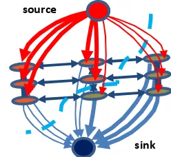
vertices or nodes, and the elements of ℰ g are called the edges of the graph G (Kropatsch et. al., 2007). Considering two special nodes, source (s) and sink (t) on a directed graph, the “minimum-cut problem” is to find a cut with minimum cost on the graph that will separate the graph into two subsets such that s is in one subset and t is in the other subset (Figure 2). The cost of a cut is the sum of all the weights of the graph edges with one node in one subset, and the other node in the other subset. Ford and Fulkerson (1962) show that considering the edge weights as capacities, finding the “maximum flow” from s to t on the same graph is equivalent to finding the “minimum cut” since a maximum flow will saturate a set of edges which will separate the graph into two disjoint parts.
Figure 2. Minimum-cut on a graph (reproduced from Boykov and Veksler, 2006)
There are numerous algorithms for solving low-level vision problems that find minimum cuts on an appropriately defined graph. Each of these algorithms has specific requirements and conditions regarding the types of energy functions they can minimize or the number of labels they can handle simultaneously. Some algorithms compute optimal solutions under certain conditions.
In this study, we adapt the fast approximate energy minimization algorithm introduced by Boykov et. al. (2001) via graph cuts and employ it for the labeling of point clouds. Their method finds a local minimum with respect to very large moves they define as 8-expansion and 8-9-swap which allow a large number of sites to change their labels simultaneously in contrast to standard moves which allow to change the label of one site at a time. They prove that the local minimum they find using 8-expansion is within a known factor of the global minimum.
s
4. CASE STUDY
4.1. Data
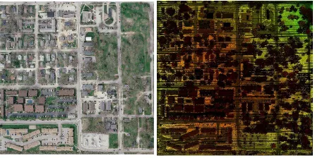
The dataset we have used to test the algorithms is the lidar point cloud of Bloomington, IN, U.S.A, obtained from the Indiana Spatial Data Portal. It is provided by Monroe County from topographic survey flights by MJ Harden on April 11-12, 2010 with an Optech Gemini system. The maximum planned post spacing on the ground is 1.4 m for unobscured areas. Reported vertical accuracy based on the accuracy assessment carried out is 0.347 ft/10.58 cm. The point cloud is provided in LAS 1.2 format. The point coordinates are in NAD 1983 HARN horizontal datum and NAVD 88 vertical datum projected on the Indiana West State Plane Coordinate System. The average point density that we have calculated from the subset of the data is 1.4 pts/m2. Figure 3 shows the study area.
Figure 3. Orthophoto (left) and height colored lidar point cloud (right) of the study area.
4.2. Point features
There are numerous feature definitions in the literature that are proposed to represent various local properties of points. Similar to surface variation, several other features are defined as a function of the eigenvalues of the covariance matrix of the point neighborhood. From these, we select to use the structure tensor planarity (S.T.P) and structure tensor anisotropy (S.T.A) features (West et. al., 2004) to identify “surface” and “scatter” points. They are defined as
:. ;. <. = = − = / = , :. ;. >. = = − = / = (5)
where = ≤ = ≤ = .
4.3. Graph construction
Adapting Boykov et. al.’s (2001) min-cut optimization algorithm, we establish our graph model as follows. Each point in the point cloud is considered as a node in the graph. The edges between the nodes are defined such that each node is connected to its 3-D voronoi neighbors with an edge. We use an edge length threshold calculated as the Euclidean 3-D distance between the two points of the edge in order to avoid very long edges and reduce the number of unnecessary edges on the graph. All points are also connected to the nodes representing labels. For each point, costs for assigning each label to that point are calculated and set as the weights for the edges that connect the points to the label nodes. These weights correspond to the data cost term of the energy function and will be summed at each candidate labeling configuration. The edges that connect points with each other are also assigned weights representing the smoothness term of the energy function. We
use two different data cost functions for two labeling tasks. The first one is for the labeling of points based on their proximity to the clusters in the feature space. It is calculated for point p as
D ?@= ‖μ − x ‖ (6)
where μ is the label mean and x is the feature vector.
In order to calculate the data costs this way, one needs to know how the data are distributed in the feature space. In a similar way to Dai and Zhang’s (2006) clustering approach for image segmentation, we perform watershed segmentation in the feature domain to empirically determine how the data are clustered. For a feature vector with N dimensions, we generate a grid space in the feature domain and calculate a histogram with the counts of data points falling within each bin. Then we perform watershed segmentation on the complement of the histogram to obtain the clusters in the feature space. We take the clusters obtained by the watershed segmentation and calculate label means from these clusters. Due to the nature of the watershed segmentation, data points that fall on the boundaries of the watersheds are left unlabeled. These data points are not considered while calculating the label means. Once the label means are determined, the data costs are calculated and the points in the point cloud are optimally assigned labels with the graph cut optimization algorithm.
The second cost function is used for labeling points with respect to their likelihood of being from a given distribution. After segmenting the points, we use the histograms of the feature values of the segments representative of their classes (i.e. “scatter” and “surface”) to calculate the data costs of assigning a point to each label as negative log likelihoods. Our feature vector consists of S.T.P. and S.T.A point features for this purpose. Data costs are calculated as
D DEFGGHI= − ln Pr-x NOPQRRST. (7)
D DUIVFEH= − ln Pr-x NOWTXQPS. (8)
Smoothness energy is calculated as
V,,-f , f,. = eZ
[\]^\_[
`a` ⋅
% ,c (9)
where d p, q is the Euclidean distance between point p and q in the spatial domain.
the algorithms in Boykov et. al. (2001), Kolmogorov and Zabih (2004), and Boykov and Kolmogorov (2004) to perform the graph cut optimization.
5. RESULTS AND DISCUSSION
We run the algorithm first for determining the “scatter” and “surface” points as described in the previous section. We set the smoothness cost parameter as σ = 0.8. We also apply weights to the data cost and smoothness cost terms to control the relative importance of conformance with the data and spatial coherence. We set E%&'& f = 1 and E ( )( f = 2. Figure 4 shows part of the study area with points labeled as “scatter” or “surface”.
Figure 4. Points color labeled as “scatter” (green) or “surface” (black) points.
Two issues may be observed regarding the effectiveness of the method. The first issue is due to small groups of points which appear to be not from a surface but being labeled as a surface point. This is mostly due to the size of the object not being large enough for identification. Second issue is related to the points that are on the ground being labeled as scatter points. This case mostly happens when those points are the lower parts of areas where there are scattered points.
After labeling points as surface and scatter, we establish a second feature vector and graph in order to segment the surface points. The first three elements of the feature vector are the components of the unit surface normal vector which is the eigenvector corresponding to the smallest eigenvalue of the covariance matrix. The last element is the surface normal variation within the point neighborhood which is the variance of the angle i between the normal vector and the vertical.
i = arccos n ⋅ o0 1 0p (10)
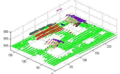
We set the number of bins to calculate the histogram for the watershed segmentation as 20 for each dimension of the feature vector. This parameter is of importance since it determines the initial clusters in the feature space. An over-segmentation is optimized by the graph cut algorithm. However, the algorithm doesn’t have the flexibility to compensate for under-segmentation as it is the case in a split and merge type of algorithm. We set the smoothness cost parameter as σ = 0.6, and the weights determining the relative importance of the smoothness and data costs as E%&'& f = 4 and E ( )( f = 1. Figure 5 shows segmented surface points in part of the study area.
6. CONCLUSION
In this study, we have established a methodology based on the graph representation of point labeling problem. We have formulated two major labeling tasks defined as an optimization
problem on graphs and employed an efficient graph cut algorithm resulting with the determination of the structure of 3-D lidar point cloud. First, we have identified the local neighborhood for each point and using the cues acquired from point neighborhood we were able to identify them as “surface” or “scatter” points. After obtaining the “surface” points, we have labeled them using a different set of features resulting in a segmentation of the surface points. Performing either of these two tasks within this framework requires prior knowledge on the structure of the feature space. Determining the distribution of the feature space for the classification problem requires some effort of collecting representative samples on the user side. However, one should note that the distribution of the features for surface and scatter points may be predicted as well.
We believe that this framework may provide better results in case the terms related to the shapes of objects like, corners, ridges, boundaries, etc. are also included in the energy function. We plan to include energy terms representing shapes and higher levels of relationships between the points within this framework in the future.
Figure 5. Color-coded point segments in part of the study area
REFERENCES
Alharthy, A. & Bethel, J., 2004. Detailed building reconstruction from airborne laser data using a moving surface method. In: The Int Arch Photogram, Rem Sens Spatial Inform
Sci, Vol XXXV, Part B3, pp.213-218.
Belton, D. & Lichti, D.D., 2006. Classification and segmentation of terrestrial laserscanner point clouds using local variance information. In: The Int Arch Photogram, Rem Sens
Spatial Inform Sci, Vol XXXVI, Part 5, pp.44-49.
Biosca, J. & Lerma, J., 2008. Unsupervised robust planar segmentation of terrestrial laser scanner point clouds based on fuzzy clustering methods. ISPRS J Photogramm, 63(1), pp.84-98.
Boykov, Y. & Kolmogorov, V., 2004. An experimental comparison of min-cut/max-flow algorithms for energy minimization in vision. IEEE transactions on pattern analysis and machine intelligence, 26(9), pp.1124-37.
Boykov, Y. & Veksler, O., 2006. Graph Cuts in Vision and Graphics: Theories and Applications. In: N. Paragios, Y. Chen,
& O. Faugeras, eds. Handbook of Mathematical Models in Computer Vision. New York: Springer US, pp. 79-96.
Pattern Analysis and Machine Intelligence, 23(11), pp.1222– 1239.
Carlberg, M. et al., 2009. Classifying urban landscape in aerial lidar using 3d shape analysis. In 16th IEEE International
Conference on Image Processing (ICIP), 2009. pp. 1701–1704.
Dai, S. & Zhang, Y., 2006. Color image segmentation in both feature and image spaces. In: Y. Zhang, ed. Advances in Image
and Video Segmentation. Herhsey: Idea, pp. 209-227
Delong, A. et al., 2010. Fast Approximate Energy Minimization with Label Costs. In IEEE Conference on Computer Vision and
Pattern Recognition (2008). pp. 1-8.
Demantke, J. et al., 2011. Dimensionality based scale selection in 3D lidar point clouds. In: The Int Arch Photogram, Rem Sens
Spatial Inform Sci, Vol XXXVIII, (5/W12).
Dey, T.K. & Goswami, S., 2004. Provable surface reconstruction from noisy samples. In: Proc. 20th Annu.
Sympos. Comput. Geom., pp.330-339.
Dorninger, P. & Nothegger, C., 2007. 3D segmentation of unstructured point clouds for building modelling. In The Int
Arch Photogram, Rem Sens Spatial Inform Sci, Vol XXXVI,
(3/W49A), pp.191–196.
Douillard, B., Underwood, J. & Kuntz, N., 2011. On the segmentation of 3D LIDAR point clouds. In Robotics and
Automation (ICRA), 2011 IEEE International Conference on.
Felzenszwalb, P.F. & Zabih, R., 2011. Dynamic Programming and Graph Algorithms in Computer Vision. IEEE Transactions on Pattern Analysis and Machine Intelligence, 33(4).
Filin, S. & Pfeifer, N., 2005. Neighborhood Systems for Airborne Laser Data. Photogramm Eng Rem S, 71(6), pp.743-755.
Filin, S. & Pfeifer, N., 2006. Segmentation of airborne laser scanning data using a slope adaptive neighborhood. ISPRS J Photogramm, 60(2), pp.71-80.
Ford, L.R., & Fulkerson, D.R., 1962. Flows in Networks. Princeton University Press, 208 pp.
Golovinskiy, A. & Funkhouser, T., 2009. Min-cut based segmentation of point clouds. In Computer Vision Workshops
(ICCV Workshops), 2009 IEEE 12th International Conference on. pp. 39-46.
Gumhold, S., Wang, X. & MacLeod, R., 2001. Feature Extraction from Point Clouds. In Proceedings of 10th
International Meshing Roundtable. pp. 293-305.
Kim, K. & Shan, J., 2011. Building roof modeling from airborne laser scanning data based on level set approach. ISPRS J Photogramm, 66(4), pp.484-497.
Kolmogorov, V. & Zabih, R., 2004. What energy functions can be minimized via graph cuts? IEEE transactions on pattern analysis and machine intelligence, 26(2), pp.147-59.
Kropatsch, W., Haxhimusa, Y. & Ion, A., 2007. Multiresolution Image Segmentations in Graph Pyramids. In A. Kandel, H. Bunke, & M. Last, eds. Springer Berlin / Heidelberg, pp. 3-41.
Lalonde, J. et al., 2005. Scale Selection for Classification of Point-Sampled 3-D Surfaces. In Fifth International Conference
on 3-D Digital Imaging and Modeling (3DIM’05). pp. 285-292.
Li, S.Z., 2009. Markov Random Field Modeling in Image Analysis, London: Springer-Verlag.
Lim, E.H. & Suter, D., 2007. Conditional Random Field for 3D Point Clouds with Adaptive Data Reduction. In 2007
International Conference on Cyberworlds (CW’07). pp.
404-408.
Mitra, N.J. & Nguyen, A., 2003. Estimating surface normals in noisy point cloud data. In Proceedings of the nineteenth
conference on Computational geometry SCG 03. ACM Press, p.
322.
Niemeyer, J., Mallet, C. & Rottensteiner, F., 2008. Conditional Random Fields for the Classification of LiDAR Point Clouds. In The Int Arch Photogram, Rem Sens Spatial Inform Sci, Vol 38 (4/W19).
OuYang, D. & Feng, H.-Y., 2005. On the normal vector estimation for point cloud data from smooth surfaces. Computer-Aided Design, 37(10), pp.1071-1079.
Pauly, M., Keiser, R. & Gross, Markus, 2003. Multi-scale Feature Extraction on Point-Sampled Surfaces. Computer Graphics Forum, 22(3), pp.281-289.
Petrie, G., & Toth, C. K., 2009. Introduction to laser ranging, profiling, and scanning. In J. Shan & C. K. Toth (Eds.),
Topographic Laser Ranging and Scanning (p. 590). Boca
Raton, FL: CRC Press
Rabbani, T., Van Den Heuvel, F. & Vosselman, G., 2006. Segmentation of point clouds using smoothness constraint. In
The Int Arch Photogram, Rem Sens Spatial Inform Sci, 36(5),
pp.1-6.
Sampath, A. & Shan, J., 2010. Segmentation and reconstruction of polyhedral building roofs from aerial lidar point clouds. Geoscience and Remote Sensing, IEEE Transactions on, 48(3), pp.1554–1567.
Szeliski, R. et al., 2008. A comparative study of energy minimization methods for Markov random fields with smoothness-based priors. IEEE transactions on pattern analysis and machine intelligence, 30(6), pp.1068-80.
Veksler, O., 1999. Efficient graph-based energy minimization methods in computer vision. Cornell Univeristy.
Vosselman, G. & Dijkman, S., 2001. 3D building model reconstruction from point clouds and ground plans. In The Int
Arch Photogram, Rem Sens Spatial Inform Sci, 34(3/W4),
pp.37–44.
Vosselman, G. et al., 2004. Recognising structure in laser scanner point clouds. In The Int Arch Photogram, Rem Sens
Spatial Inform Sci, 46(8), pp.33-38.