ELECTRONIC COMMUNICATIONS in PROBABILITY
EXPONENTIAL BOUNDS FOR MULTIVARIATE SELF-NORMALIZED
SUMS
PATRICE BERTAIL
Laboratory of Statistics, CREST and MODALX, University Paris X, France email: [email protected]
EMMANUELLE GAUTHERAT
Laboratory of Statistics, CREST and Economic Faculty of Reims, France email: [email protected]
HUGO HARARI-KERMADEC
Laboratory of Statistics, CREST, Timbre J340, 3 av. P. Larousse, 92241 Malakoff Cedex and Université Paris-Dauphine, France
email: [email protected]
SubmittedApril 9, 2008, accepted in final formNovember 25, 2008 AMS 2000 Subject classification: Primary 62G15 ; secondary 62E17, 62H15.
Keywords: Exponential inequalities; Self-normalization; multivariate; Hoeffding inequality.
Abstract
In a non-parametric framework, we establish some non-asymptotic bounds for self-normalized sums and quadratic forms in the multivariate case for symmetric and general random variables. This bounds are entirely explicit and essentially depends in the general case on the kurtosis of the Euclidean norm of the standardized random variables.
1
Introduction
LetZ,Z1, ...,Znbe i.i.d. random centered vectors from a probability space (Ω,A, Pr)to (Rq,B,P).
We denoteEthe expectation underP. In the following we putZ
n=n−1
Pn
i=1Zi. DefineSa square root of the matrixS2=E(Z Z′)and similarlyS
na square root ofSn2=n−
1Pn
i=1ZiZ ′
i. We assume in the following thatS2is full rank and thereforeS2
nis also full rank with probability 1 as soon as n>p. For further use, we defineγr =E(kS−1Zkr
2), r>0, where|| ||2is the Euclidean norm on
Rq. Now consider the self-normalized sum
n1/2Sn−1Zn= n
X
i=1
ZiZi′
!−1/2 n X
i=1
Zi. (1)
and its Euclidean norm
nZ′nSn−2Zn (2)
Self-normalized sums have recently given rise to an important literature : see for instance[13, 6]
or[4]for self-normalized processes. It has been proved that non-asymptotic exponential bounds can be obtained for these quantities under very weak conditions on the underlying moments of the variablesZi. Unfortunately, except in the symmetric case, these bounds established in the real case (q=1)are not universal and depend on the skewnessγ3=E|S−1Z|3or even an higher moments
for instanceγ10/3=E|S−1Z|10/3, see[13]. Actually, uniform bounds inPare impossible to obtain,
otherwise this would contradict Bahadur and Savage’s Theorem, see [2, 18]. Recall that the behaviour of self-normalized sums is closely linked to the behaviour of the statistics of Student, which is the basic asymptotic root for constructing confidence intervals (see Remark 2 below). Moreover, available bounds are not explicit and only valid forn≥n0,n0large and unknown. To
our knowledge, non-asymptotic exponential bounds withexplicit constantsare only available for symmetric distribution[12, 9, 17], in the unidimensional case (q=1). In this paper, we obtain generalizations of these bounds for (2) in the multivariate case by using a multivariate extension of the symmetrization method developed in[16]as well as arguments taken from the literature on self-normalized process, see[4]. Our bounds are explicit but depend on the kurtosisγ4of the Euclidean norm ofS−1Zrather than on the skewness. They hold for any value of the parameter sizeq. One technical difficulty in the multidimensional case is to obtain an explicit exponential bound for the smallest eigenvalue of the empirical variance which allows to control the deviation ofS2
nfromS
2, a result which has its own interest.
2
Exponential bounds for self-normalized sums
Some bounds for self-normalized sums may be quite easily obtained in the symmetric case (that is for random variables having a symmetric distribution) and are well-known in the unidimensional case. In non-symmetric and/or multidimensional case theses bounds are new and not trivial to prove. One of the main tools for obtaining exponential inequalities in various setting is the famous Hoeffding inequality (see[12]) yielding that for independent real random variables (r.v.) Yi,i=1, ...,n, with finite support say[0, 1], we have
Pr
n−1
n
X
i=1
Yi
!2
≥t
≤2 exp
−2t
.
A direct application of this inequality to self-normalized sums (via a randomization step introduc-ing Rademacher r.v.’s) yields (see[9, 8]) that, fornindependent random variablesZi symmetric about 0, and not necessarily bounded (nor identically distributed), we have
Pr
Pn i=1Zi
2 Pn
i=1Zi2
≥t
≤2 exp
−t
2
. (3)
In the general non-symmetric case, the master result of[13]forq=1 states that ifγ10/3<∞,
then for someA∈Rand somea∈]0, 1[,
Pr
Pn i=1Zi
2 Pn
i=1Z 2
i
≥t
where Fq is the survival function of a χ2(q)distribution defined by F
q(t) =
R+∞
t fq(y)d y with fq(y) =
1 2q/2Γ(q/2)y
q/2−1e−y2 andΓ(p) =
R+∞
0 y
p−1e−yd y.
However the constantsAandaare not explicit and, despite of its great interest to understand the large deviation behaviour of self-normalized sums, the bound is of no direct practical use. In the non-symmetric case our bounds are worse than (4) as far as the control of the approximation by a
χ2(q)distribution are concerned, but entirely explicit.
Theorem 1. Let Z, (Zi)1≤i≤n, be an i.i.d. sample inRq with probabilityP. Suppose that S2is of
rank q. Then the following inequalities hold,for finiten>q and for t<nq,
a) if Z has a symmetric distribution, then, without any moment assumption, Pr
nZ′nS−n2Zn≥t
≤2qe−2tq; (5)
b) for general distribution of Z,withγ4<∞, for any a>1,
Pr
nZ′nSn−2Zn≥t
≤2qe1−2q(1+t a)+C(q)n3˜qγ−˜q
4 e
− n
γ4(q+1)
1−1
a
2
(6)
≤2qe1−2q(1+t a)+K(q)n3˜qe−
n
γ4(q+1)
1−1
a
2
with˜q=q−1 q+1and
C(q) = (2eπ)
2˜q(q+1)
22/(q+1)(q−1)3˜q and K(q) = C(q)
q2˜q ≤8. Moreover for nq≤t, we have
PrnZ′nSn−2Zn≥t=0.
The proof is postponed to Appendix (1). Part a) in the symmetric multidimensional case follows by an easy but crude extension of[12]or[9, 8]. It is also given under a different form in[10]. The exponential inequality (5) is classical in the unidimensional case. Other type of inequalities with suboptimal rate in the exponential term have also been obtained by[14].
In the general multidimensional framework, the main difficulty is actually to keep the self-normalized structure when symmetrizing the original sum. We first establish the inequality in the symmet-ric case by an appropriate diagonalization of the estimated covariance matrix, which reduces the problem to q -unidimensional inequalities. The next step is to use a multidimensional version of Panchenko’s symmetrization lemma (see[16]). However this symmetrization lemma destroys partly the self-normalized structure (the normalization is thenS2
n+S2instead of the expectedSn2), which can be retrieved by obtaining a lower tail control of the distance betweenS2
n andS2. This is done by studying the behavior of the smallest eigenvalue of the normalizing empirical variance. The second term in the right hand side of inequality (6) is essentially due to this control.
χ2(q)distribution. Notice that this tail F
qsatisfies the following approximation (see[1], p. 941, result 26.4.12 )
Fq(t)t∼ →∞
1 Γ(q
2) t
2
q
2−1 exp(−t
2).
This bounds gives the right behavior of the tail (in q) as t grows, which is not the case for a). However, in the unidimensional case a) still gives a better approximation than[17]. a) can still be used in the multidimensional case to get crude but exponential bounds. We expect however Pinelis’ inequality to give much better bounds for moderateq and moderate sample sizenin the symmetric case. For these reason, we will extend the results of Theorem 1 by using aχ2(q)type
of control. This essentially consists in extending Lemma 1 of[16]to non exponential bound.
Theorem 2. The following inequalities hold,for finiten>q and for t<nq:
a) (Pinelis 1994) if Z has a symmetric distribution, without any moment assumption, then we have
Pr
nZ′nSn−2Zn≥t
≤ 2e
3
9 Fq(t), (7)
b) for general distribution of Z with kurtosisγ4<∞, for any a>1and for t ≥2q(1+a)and ˜
q= q−1
q+1 we have
Pr
nZ′nS−n2Zn≥t
≤ 2e
3
9Γ(q
2+1)
t−q(1+a) 2(1+a)
q
2 e−
t−q(1+a) 2(1+a) +C(q)
n3
γ4
˜q e−
n(1−1a)
2
γ4(q+1)
≤ 2e
3
9Γ(q
2+1) t
−q(1+a) 2(1+a)
q
2 e−
t−q(1+a)
2(1+a) +K(q)n3˜qe−
n(1−1a)
2
γ4(q+1) (8)
For t≥nq, we havePr
nZ′nS−2
n Zn≥t
=0.
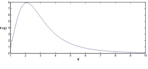
Remark 1. Notice that the constant K(q)does not increase with large q as it can be seen on Figure 1. A close examination of the bounds shows that essentiallyγ4(q+1)has to be small compared to n
1 2 3 4 5 6 7 8 9 10
0 1 2 3 4 5 6 7 8
q K(q)
Figure 1: Value ofK(q)as a function ofq
Remark 2. It can be tempting to compare our bounds with some more classical results in statistics. We recall that, in an unidimensional framework, the studentized ratio is given byTen=pneS−n1Z¯nwhere
e
Snis the unbiased estimator of the varianceeSn= (n−11
Pn
i=1(Zi−Z¯n)2)−1/2. In a Gaussian framework,
e
Tnhas a Student distribution with(n−1)degrees of freedom. In opposition, our self-normalized sum is defined by Tn = pn
1
n
Pn i=1Z
2
i
−1/2
¯
Zn. It is related to Ten by the relation Tn = fn(Ten) with fn(x) =
p n
n−1
1+ x2 n−1
−1/2
x. As a consequence, one gets in an unidimensional symmetric case, for t>0,
Pr(Ten≥t)≤exp
−
1 2
n n−1
t2
1+ t2 n−1
.
For large n we recover an sub-gaussian type of inequality. At fixed n, , this inequality is noninformative for t → ∞ since the right-hand side tends to 1. Recall that, in a Gaussian framework, the tail P r(Ten>t)is of order O( 1
tn−1)as t→ ∞.
Remark 3. In the best case, past studies give some bounds for n sufficiently large, without an exact value for ”sufficiently large”. Here, the bounds are valid and explicit for any n>q.
These bounds are motivated by some statistical applications to the construction of non-asymptotic confidence intervals with conservative coverage probability in a semi-parametric setting. Self-normalized sums appear naturally in the context of empirical likelihood and its generalization to Cressie-Read divergences, see[11, 15]. In particular, [5]shows how the bounds obtained here may be used to construct explicit non asymptotic confidence regions, even whenqdepends onn.
A
Proofs of the main results
A.1
Some lemmas
The first lemma is a direct extension of Panchenko, 2003, Corollary 1 to the multidimensional case, which will be used both in theorem 1 and 2.
Lemma 1. LetJq be the unit sphere ofRq, Jq ={λ ∈Rq, kλk2 =1}. Let Z(n) = (Zi)1≤i≤nand Y(n)= (Yi)1≤i≤nbe i.i.d. centered random vectors inRqwith Z(n)independent of Y(n). We denote, for any random vector W= (Wi)1≤i≤nwith coordinates inRq, Sn2,W=
1
n
Pn iWiWi′. If there exists D>0and d>0such that, for all t≥0,
Pr
sup
λ∈Jq
p
nλ′(Z n−Yn)
Æ
λ′S2
n,(Z(n)−Y(n))λ
≥pt
≤De−d t, (9)
then, for all t≥0,
Pr
sup
λ∈Jq
p
nλ′Zn
p
λ′S2
nλ+λ′S2λ
≥pt
Proof. This proof follows Lemma 1 of[16]with some adaptations to the multidimensional case. Denote
An(Z(n)) =sup
λ∈Jq
sup b>0 n
E
h
4b(λ′(Zn−Yn)−bλ′S2n,Z(n)
−Y(n)λ)|Z
(n)io
Cn(Z(n),Y(n)) =sup
λ∈Jq
sup b>0 n
4b(λ′(Zn−Yn)−bλ′S2
n,Z(n)−Y(n)λ)
o
.
By Jensen inequality, we have Pr-almost surely
An(Z(n))≤E[Cn(Z(n),Y(n))|Z(n)] and, for any convex functionΦ, by Jensen inequality, we also get
Φ(An(Z(n)))
≤E[Φ(Cn(Z(n),
Y(n)))|Z(n)]. We obtain
E(Φ(An(Z(n))))
≤E(Φ(Cn(Z(n),
Y(n)))). (11)
Now remark that
An(Z(n)) = sup
λ∈Jq
sup b>0 ¦
4bλ′Z
n−bλ′Sn2λ−bλ′S
2λ©
= sup
λ∈Jq
λ′Zn
p
λ′S2
nλ+λ′S2λ
2
and
Cn(Z(n),Y(n)) = sup
λ∈Jq
λ
′(Z n−Yn)
Æ
λ′S2
n,Z(n)−Y(n)λ
2
.
Now, notice that supλ∈Jq
λ′Z
n
p
λ′S2
nλ
>0 and apply the arguments of the proof of[16]’s Corollary 1
applied to inequality (11) to obtain the result.
The next lemma allows to establish an non exponential version of the preceding lemmas. Indeed a consequence of this lemma is that, if the tail of the symmetrized version in inequality (9) is con-trolled by a chi-square tail, then the non symmetrized version may be concon-trolled by an exponential multiplied by a polynomial. The rate in the exponential is asymptotically correct.
Lemma 2. For any t>q, letΦt(x) =max(x−t+q; 0). Letνandξbe two r.v.’s, such that for any t>q, EΦt(ξ)≤EΦt(ν). Suppose that, there exists a constant C>0such that, for t>0,
Pr(ν >t)≤C Fq(t). Then, for t≥2q, we have
Pr(ξ >t)≤C
(t −q)
2
q
2 e− (t−q)
2
Γ(q/2+1).
and for t>q, we have
Proof. We follow the lines of the proof of Panchenko’s lemma, with function Φt. Remark that Φt(0) =0 andΦt(t) =q, then we have
Pr(ξ≥t) ≤ 1 Φt(t)
Φt(0) +
Z+∞
0
Φ′t(x)Pr(ν≥x)d x
!
≤ C
q
Z+∞
t−q
Fq(x)d x.
By integration by parts, we have
Z+∞
t−q
Fq(x)d x=
Z+∞
t−q
x fq(x)d x−(t−q)
Z+∞
t−q
fq(x)d x.
It follows by straightforward calculations that, for t>q,
Pr(ξ≥t) ≤ C q
Z+∞
t−q
Fq(x)d x≤C
Fq+2(t−q)−
t−q
q Fq(t−q)
.
Fort≥2q, and using the recurrence relation 26.4.8 of[1], page 941.
Pr(ξ≥t) ≤ CFq+2(t−q)−Fq(t−q)
=
(t−q) 2
q/2 C e−(t−2q) Γ(q
2+1)
.
Moreover, for t>qwe have Pr(ξ≥t)≤C Fq+2(t−q).
We now extend a result of [3], which controls the behavior of the smallest eigenvalue of the empirical variance. In the following, for a given symmetric matrixA, we denoteµ1(A)its smallest eigenvalue.
Lemma 3. Let (Zi)1≤i≤n be i.i.d. random vectors inRq with common mean0. Assume1≤ eγ4= E(kZ1k4
2)<+∞. Then, for any n>q and0<t≤µ1(S2),
Prµ1(S2n)≤t
≤C(q)n
3eqµ
1(S2)2˜q e
γ˜q4 exp
−n(µ1(S 2)−t)2 e
γ4(q+1)
∧1,
witheq= q−1 q+1 and
C(q) =π2˜q(q+1)e2˜q(q−1)−3˜q22˜q−q+12 (12)
≤4π2(q+1)e2(q−1)−3˜q. (13)
Proof. The proof of this result is adapted from[3]and makes use of some idea of[4].
We first have by a truncation argument and applying Markov’s inequality on the last term in the inequality (see the proof of[3], Lemma 4), for everyM>0,
Pr µ1
n
X
i=1
ZiZi′
! ≤nt
!
≤Pr inf v∈Jq
n
X
i=1
(v′Zi)2≤nt, sup i=1,...,n||
Zi||2≤M
!
+neγ4
We callI the first term on the right hand side of this inequality.
Notice that by symmetry of the sphere, we can always work with the northern hemisphere of the sphere rather than the sphere. In the following, we denote byNq the northern hemisphere of the sphere. Notice that, if the supremum of the||Zi||2is smaller thanM, then foru,vinNq, we have
¯ ¯ ¯ ¯ ¯
n
X
i=1
(v′Zi)2− n
X
i=1
(u′Zi)2
¯ ¯ ¯ ¯
¯≤2n||u−v||2M 2.
Thus ifuandvare apart by at mosttη/(2M2)then|Pn
i=1(v′Zi)2−
Pn
i=1(u′Zi)2| ≤ηnt. Now let N(Nq,ǫ)be the smallest number of caps of radiusǫcentered at some points onNq (for the||.||2 norm) needed to coverNq. Now we follow the same arguments as[3]to controlI: I is bounded by the sum of the probabilities that the infimum ofPni=1(v′Z
i)2 over each cap is smaller thant nt and that supi=1,...,n||Zi||2 ≤ M. We bound this sum by the number of caps times the larger probability: for anyη >0,
I ≤N
Nq,
tη
2M2
max u∈Nq
Pr n
X
i=1
(u′Z
i)2≤(1+η)nt
!
.
The proof is now divided in three steps, i) control ofN(Nq,2tMη2), ii) control of the maximum over
Nq of the last expression inI, iii) optimization over all the free parameters.
i) On the one hand, we have, for some constantb(q)>0,
N(Nq,ǫ)≤b(q)ǫ−(q−1)
∨1. (15)
For instance, we may choose b(q) =πq−1. Indeed, following[3], the northern hemisphere can
be parameterized in polar coordinates, realizing a diffeomorphism withJq−1×[0,π]. Now pro-ceed by induction, notice that forq=2,Nq, the half circle can be covered by[π/2ǫ]∨1+1≤ 2([π/2ǫ]∨1) ≤π/ǫ∨1 caps of diameter 2ǫ, that is, we can choose the caps with their cen-ter on aǫ−grid on the circle. Now, by induction we can cover the cylinder Jq−1×[0,π] with [π/2ǫ(π)q−2/ǫq−2]∨1+1≤πq−1/ǫq−1intersecting cylinders which in turn can be mapped to
region belonging to caps of radiusǫ, covering the whole sphere (this is still a covering because the mapping from the cylinder to the sphere is contractive).
ii) On the other hand, for all t > 0, we have by exponentiation and Markov’s inequality, and independence of(Zi)1≤i≤n, for anyλ >0
max u∈Nq
Pr n
X
i=1
u′ZiZi′u≤nt
!
≤enλtmax u∈Nq
Ee−λu′Z1Z1′u
Now, using the classical inequalities, log(x)≤x−1 ande−x−1≤ −x+x2/2, both valid forx>0,
We now optimize inM2>0 and the optimum is attained at
M∗2=
Using the constant b(q) =πq−1we get the expression ofC(q), which is bounded by the simpler
bound (for large q this bound will be sufficient) 4π2(q+1)e2(q−1)−3qq−1+1
A.2
Proof of Theorem 1
Proof. Notice that we have always ¯Zn′S−n2Z¯n≤q. Indeed, there exists an orthogonal transformation Onand a diagonal matrixΛ2n:=diag[ ˆµj]1≤j≤q withµˆj>0 being the eigenvalues ofS2n, such that
This quantity is lower thanqby Cauchy-Schwartz inequality. So, it follows that, for allt>qn PrnZ¯n′Sn−2Z¯n≥t
=0.
a) In the symmetric and unidimensional framework (q=1), this bound follows from Hoeffding inequality (see [9]). Consider now the symmetric multidimensional framework (q > 1). Let
σi, 1 ≤ i ≤ n be Rademacher random variables, independent from (Zi)1≤i≤n, P(σi = −1) = theZi’s have a symmetric distribution, meaning that−Zihas the same distribution asZi, we make use of a first symmetrization step:
Pr
b) TheZi’s are not anymore symmetric. Define
First of all, remark that the following events are equivalent
n
The control of the first term on the right hand side is obtained in two steps. First apply part a) of
Theorem 1 ton1/2sup
. Then, by application of Lemma 1 and (18), we get
A.3
Proof of Theorem 2.
Part a) is proved in [17]. Now, the proof of part b) follows the same lines as the Theorem 1 combining Lemmas 1, 2 and 3.
References
[1] M. Abramovitch and L. A. Stegun. Handbook of Mathematical Tables. National Bureau of Standards, Washington, DC, 1970.
[2] R. R. Bahadur and L. J. Savage. The nonexistence of certain statistical procedures in non-parametric problems. Annals of Mathematical Statistics, 27:1115–1122, 1956. MR0084241
[3] P. Barbe and P. Bertail. Testing the global stability of a linear model. Working Paper nˇr46, CREST, 2004.
[4] B. Bercu, E. Gassiat, and E. Rio. Concentration inequalities, large and moderate deviations for self-normalized empirical processes. Annals of Probability, 30(4):1576–1604, 2002. MR1944001
[5] P. Bertail, E. Gauthérat, and H. Harari-Kermadec. Exponential bounds for quasi-empirical likelihood. Working Paper nˇr34, CREST, 2005.
[6] G. P. Chistyakov and F. Götze. Moderate deviations for Student’s statistic. Theory of Proba-bility & Its Applications, 47(3):415–428, 2003.
[7] M. L. Eaton. A probability inequality for linear combinations of bounded random variables. Annals of Statistics, 2:609–614, 1974.
[8] M. L. Eaton and B. Efron. Hotelling’st2test under symmetry conditions. Journal of ameri-can statistical society, 65:702–711, 1970. MR0269021
[9] B. Efron. Student’st-test under symmetry conditions.Journal of american statistical society, 64:1278–1302, 1969. MR0251826
[10] E. Giné and F. Götze. On standard normal convergence of the multivariate Student t-statistic for symmetric random vectors. Electron. Comm. Probab., 9:162–171 (electronic), 2004. ISSN 1083-589X. MR2108862
[11] H. Harari-Kermadec. Vraisemblance empirique généralisée et estimation semi-paramétrique. PhD thesis, Université Paris X, 2006.
[12] W. Hoeffding. Probability inequalities for sums of bounded variables.Journal of the Ameri-can Statistical Association, 58:13–30, 1963. MR0144363
[13] B.-Y. Jing and Q. Wang. An exponential nonuniform Berry-Esseen bound for self-normalized sums.Annals of Probability, 27(4):2068–2088, 1999. MR1742902
[14] P. Major. A multivariate generalization of Hoeffding’s inequality. Arxiv preprint math. PR/0411288, 2004.
[16] D. Panchenko. Symmetrization approach to concentration inequalities for empirical pro-cesses. Annals of Probability, 31(4):2068–2081, 2003. MR2016612
[17] I. Pinelis. Probabilistic problems and Hotelling’st2test under a symmetry condition.Annals of Statistics, 22(1):357–368, 1994. MR1272088