Chapter XX
Chapter Outline
Chapter Outline
1) Overview
1) Overview
2) Basic Concept
2) Basic Concept
3) Statistics Associated with Cluster Analysis
3) Statistics Associated with Cluster Analysis
4) Conducting Cluster Analysis
4) Conducting Cluster Analysis
i. Formulating the Problem
i. Formulating the Problem
ii. Selecting a Distance or Similarity Measure
ii. Selecting a Distance or Similarity Measure
iii. Selecting a Clustering Procedure
iii. Selecting a Clustering Procedure
iv. Deciding on the Number of Clusters
iv. Deciding on the Number of Clusters
v. Interpreting and Profiling the Clusters
v. Interpreting and Profiling the Clusters
5) Applications of Nonhierarchical Clustering
5) Applications of Nonhierarchical Clustering
6) Clustering Variables
6) Clustering Variables
7) Internet & Computer Applications
7) Internet & Computer Applications
8) Focus on Burke
8) Focus on Burke
9) Summary
9) Summary
10) Key Terms and Concepts
10) Key Terms and Concepts
11) Acronyms
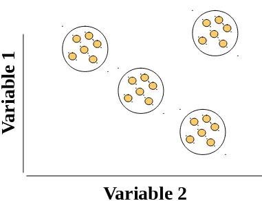
An Ideal Clustering Situation
An Ideal Clustering Situation
Figure 20.1
Figure 20.1
Variable 2
V
ar
ia
b
le
X
X
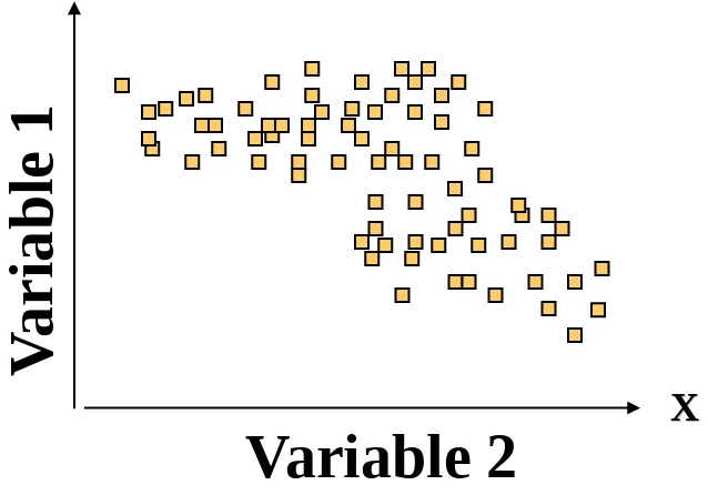
A Practical Clustering Situation
[image:5.720.194.513.188.411.2]A Practical Clustering Situation
Figure 20.2
Figure 20.2
Variable 2
V
ar
ia
b
le
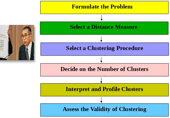
Conducting Cluster Analysis
Conducting Cluster Analysis
Fig. 20.3
Fig. 20.3
Select a Distance Measure
Formulate the Problem
Select a Clustering Procedure
Decide on the Number of Clusters
Interpret and Profile Clusters
Case No.
V
1V
2V
3V
4V
5V
61
6
4
7
3
2
3
2
2
3
1
4
5
4
3
7
2
6
4
1
3
4
4
6
4
5
3
6
5
1
3
2
2
6
4
6
6
4
6
3
3
4
7
5
3
6
3
3
4
8
7
3
7
4
1
4
9
2
4
3
3
6
3
10
3
5
3
6
4
6
11
1
3
2
3
5
3
12
5
4
5
4
2
4
13
2
2
1
5
4
4
14
4
6
4
6
4
7
15
6
5
4
2
1
4
16
3
5
4
6
4
7
17
4
4
7
2
2
5
18
3
7
2
6
4
3
19
4
6
3
7
2
7
20
2
3
2
4
7
2
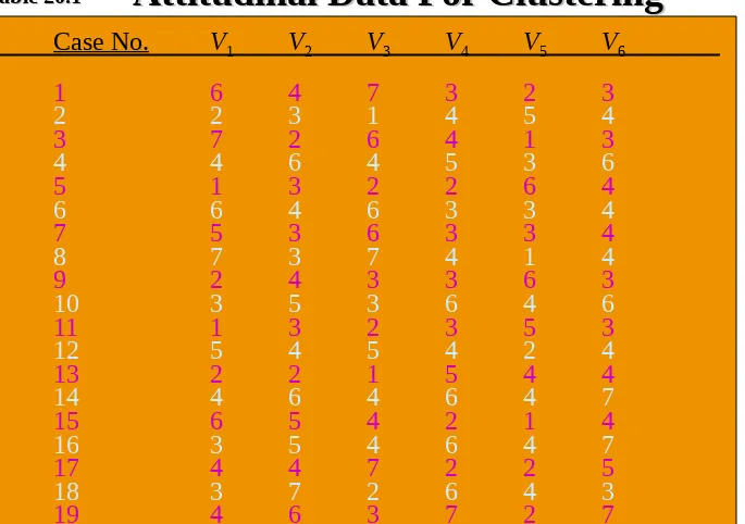
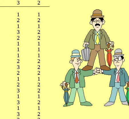
[image:7.720.35.720.41.523.2]Attitudinal Data For Clustering
Attitudinal Data For Clustering
Table 20.1
Fig. 20.4
Fig. 20.4
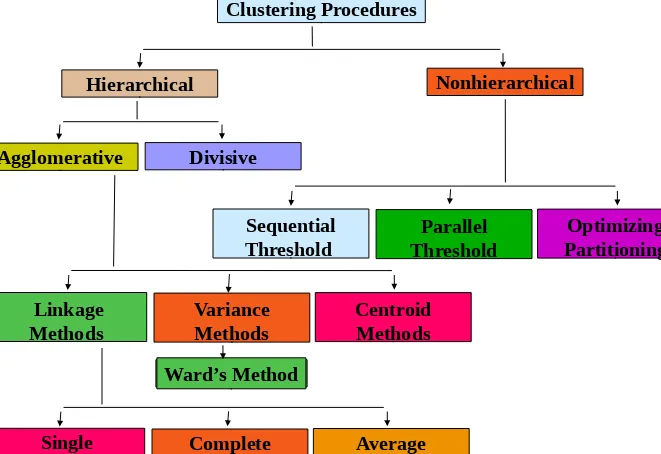
Clustering Procedures
A Classification of Clustering Procedures
A Classification of Clustering Procedures
Hierarchical
Nonhierarchical
Agglomerative
Divisive
Sequential
Threshold
Parallel
Threshold
Optimizing
Partitioning
Linkage
Methods
Variance
Methods
Centroid
Methods
Ward’s Method
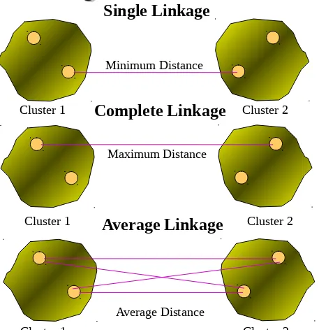
Linkage Methods of Clustering
Linkage Methods of Clustering
Figure 20.5
Figure 20.5
Single Linkage
Minimum Distance
Complete Linkage
Maximum Distance
Average Linkage
Average Distance
Cluster 1 Cluster 2
Cluster 1 Cluster 2
Other Agglomerative Clustering Methods
Other Agglomerative Clustering Methods
Fig. 20.6Fig. 20.6
Ward’s Procedure
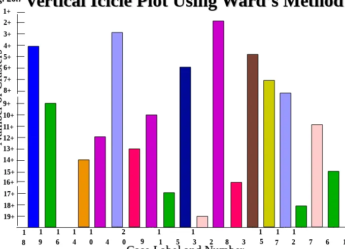
Vertical Icicle Plot Using Ward’s Method
Vertical Icicle Plot Using Ward’s Method
Fig. 20.7Fig. 20.7
1 1 1 1 1 2 1 1 1 1 1
8+ 1+ 4+ 5+ 6+ 7+ 2+ 3+ 11+ 12+ 13+ 14+ 9+ 10+ 16+ 19+ 17+ 18+ 15+ 9
8 9 6 4 0 4 0 1 5 3 2 8 3 5 7 2 7 6 1
Case Label and Number
Case Label and Number
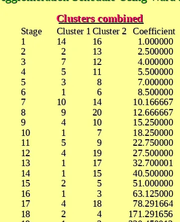
Results of Hierarchical Clustering
Results of Hierarchical Clustering
Table 20.2
Table 20.2
Stage cluster
Stage cluster
Clusters combined
Clusters combined
first appears
first appears
Stage
Stage Cluster 1Cluster 1Cluster 2Cluster 2 Coefficient Cluster 1 Cluster 2 Next stage Coefficient Cluster 1 Cluster 2 Next stage 1
1 1414 1616 1.000000 1.000000 0 0 0 0 7 7 2
2 2 2 1313 2.500000 2.500000 0 0 0 0 15 15 3
3 7 7 1212 4.000000 4.000000 0 0 0 0 10 10 4
4 5 5 1111 5.500000 5.500000 0 0 0 0 11 11 5
5 3 3 8 8 7.000000 7.000000 0 0 0 0 16 16 6
6 1 1 6 6 8.500000 8.500000 0 0 0 0 10 10 7
7 1010 1414 10.166667 10.166667 0 0 1 1 9 9 8
8 9 9 2020 12.666667 12.666667 0 0 0 0 11 11 9
9 4 4 1010 15.250000 15.250000 0 0 7 7 12 12 10
10 1 1 7 7 18.250000 18.250000 6 6 3 3 13 13 11
11 5 5 9 9 22.750000 22.750000 4 4 8 8 15 15 12
12 4 4 1919 27.500000 27.500000 9 9 0 0 17 17 13
13 1 1 1717 32.700001 32.700001 1010 0 0 14 14 14
14 1 1 1515 40.500000 40.500000 1313 0 0 16 16 15
15 2 2 5 5 51.000000 51.000000 2 2 1111 18 18 16
16 1 1 3 3 63.125000 63.125000 1414 5 5 19 19 17
17 4 4 1818 78.291664 78.291664 1212 0 0 18 18 18
18 2 2 4 4 171.291656171.291656 1515 1717 19 19 19
19 1 1 2 2 330.450012330.450012 1616 1818 0 0
Agglomeration Schedule Using Ward’s Procedure
Number of Clusters
Number of Clusters
Label case
Label case 44 33 22 1
1 11 11 11
2
2 22 22 22
3
3 11 11 11
4
4 33 33 22
5
5 22 22 22
6
6 11 11 11
7
7 11 11 11
8
8 11 11 11
9
9 22 22 22
10
10 33 33 22
11
11 22 22 22
12
12 11 11 11
13
13 22 22 22
14
14 33 33 22
15
15 11 11 11
16
16 33 33 22
17
17 11 11 11
18
18 44 33 22
19
19 33 33 22
20
20 22 22 22
Cluster Membership of Cases Using Ward’s Procedure
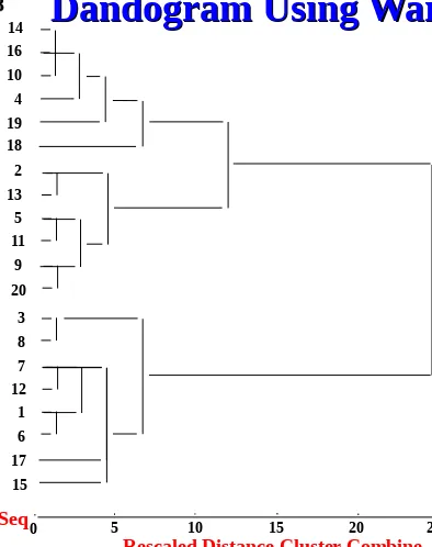
[image:13.720.197.648.85.501.2]Dandogram Using Ward’s Method
[image:14.720.92.486.28.526.2]Dandogram Using Ward’s Method
Fig. 20.8
Fig. 20.8
3
15 1 12 7 8
17 6 11 5 13 2
20 9 19 16
4 10
18 14
0 5 10 15 20 25
Case Label Seq
Means of Variables
Cluster No.
V
1V
2V
3V
4V
5V
61 5.750 3.625 6.000 3.125 1.750 3.875
2 1.667 3.000 1.833 3.500 5.500 3.333
3 3.500 5.833 3.333 6.000 3.500 6.000
Cluster
[image:15.720.36.714.79.502.2]Cluster
Centroids
Centroids
Table 20.3
Cluster
Cluster V1V1 V2V2 V3V3 V4V4 V5V5 V6V6 1
1 4.00004.0000 6.00006.0000 3.00003.0000 7.00007.0000 2.00002.0000 7.00007.0000 2
2 2.00002.0000 3.00003.0000 2.00002.0000 4.00004.0000 7.00007.0000 2.00002.0000 3
3 7.00007.0000 2.00002.0000 6.00006.0000 4.00004.0000 1.00001.0000 3.00003.0000
Initial Cluster Centers
Initial Cluster Centers
[image:16.720.12.604.68.531.2]Results of Nonhierarchical Clustering
Results of Nonhierarchical Clustering
Table 20.4
Table 20.4
Classification Cluster Centers
Classification Cluster Centers
Cluster
Cluster V1V1 V2V2 V3V3 V4V4 V5V5 V6V6 1
1 3.81353.8135 5.89925.8992 3.25223.2522 6.48916.4891 2.51492.5149 6.69576.6957 2
2 1.85071.8507 3.02343.0234 1.83271.8327 3.78643.7864 6.44366.4436 2.50562.5056 3
3 6.35586.3558 2.83562.8356 6.15766.1576 3.67363.6736 1.30471.3047 3.20103.2010
Case Listing of Cluster Membership
Case Listing of Cluster Membership
Case ID
Case ID ClusterCluster DistanceDistance Case IDCase ID ClusterCluster DistanceDistance 1
1 33 1.7801.780 22 22 2.2542.254 3
3 33 1.1741.174 44 11 1.8821.882 5
5 22 2.5252.525 66 33 2.3402.340 7
7 33 1.8621.862 88 33 1.4101.410 9
9 22 1.8431.843 1010 11 2.1122.112 11
11 22 1.9231.923 1212 33 2.4002.400 13
13 22 3.3823.382 1414 11 1.7721.772 15
15 33 3.6053.605 1616 11 2.1372.137 17
17 33 3.7603.760 1818 11 4.4214.421 19
Final Cluster Centers
Final Cluster Centers
Table 20.4 contd.
Table 20.4 contd.
Cluster
Cluster V1V1 V2V2 V3V3 V4V4 V5V5 V6V6 1
1 3.50003.5000 5.83335.8333 3.33333.3333 6.00006.0000 3.50003.5000 6.00006.0000 2
2 1.66671.6667 3.00003.0000 1.83331.8333 3.50003.5000 5.50005.5000 3.33333.3333 3
3 5.75005.7500 3.62503.6250 6.00006.0000 3.12503.1250 1.75001.7500 3.87503.8750
Distances between Final Cluster Centers
Distances between Final Cluster Centers
Cluster
Cluster 1 1 2 2 3 3 1
1 0.00000.0000 2
2 5.56785.5678 0.00000.0000 3
3 5.73535.7353 6.99446.9944 0.00000.0000
Analysis of Variance
Analysis of Variance
Variable
Variable Cluster MS df Error MS df F p Cluster MS df Error MS df F p V1
V1 29.1083 29.1083 22 0.60780.6078 17 47.8879 .000 17 47.8879 .000 V2
V2 13.5458 13.5458 22 0.62990.6299 17 21.5047 .000 17 21.5047 .000 V3
V3 31.3917 31.3917 22 0.83330.8333 17 37.6700 .000 17 37.6700 .000 V4
V4 15.7125 15.7125 22 0.72790.7279 17 21.5848 .000 17 21.5848 .000 V5
V5 24.1500 24.1500 22 0.73530.7353 17 32.8440 .000 17 32.8440 .000 V6
V6 12.1708 12.1708 22 1.07111.0711 17 11.3632 .001 17 11.3632 .001
Number of Cases in each Cluster
Number of Cases in each Cluster
Cluster
Cluster Unweighted Cases Unweighted Cases Weighted Cases Weighted Cases 1
1 6 6 66
2
2 6 6 66
3
3 8 8 88
Missing
Missing 0 0
Total
How do consumers in different countries perceive brands in
different product categories? Surprisingly, the answer is that the
product perception parity rate is quite high. Perceived product
parity means that consumers perceive all/most of the brands in a
product category as similar to each other or at par. A new study
by BBDO Worldwide shows that two-thirds of consumers
surveyed in 28 countries considered brands in 13 product
categories to be at parity. The product categories ranged from
airlines to credit cards to coffee.
Perceived Product Parity - Once
Rarity - Now Reality
RIP 20.1
Perceived parity averaged 63% for all
categories in all countries. The Japanese
have the highest perception of parity
across all product categories at 99% and
Colombians the lowest at 28%. Viewed by
product category, credit cards have the
highest parity perception at 76% and
cigarettes the lowest at 52%.
BBDO clustered the countries based on
product parity perceptions to arrive at
clusters that exhibited similar levels and
The highest perception parity figure came from Asia/Pacific region
(83%) which included countries of Australia, Japan, Malaysia, and
South Korea, and also France. It is no surprise that France was in this
list since for most products they use highly emotional, visual
advertising that is feelings oriented. The next cluster was
U.S.-influenced markets (65%) which included Argentina, Canada, Hong
Kong, Kuwait, Mexico, Singapore, and the U.S. The third cluster,
primarily European countries (60%) included Austria, Belgium,
Denmark, Italy, the Netherlands, South Africa, Spain, the U.K., and
Germany.
RIP 20.1 Contd.
What all this means is that in order to
differentiate the product/brand,
advertising can not just focus on product
performance, but also must relate the
product to the person's life in an
important way. Also, much greater
marketing effort will be required in the
Asia/Pacific region and in France in
order to differentiate the brand from
competition and establish a unique
image. A big factor in this growing parity
Cluster analysis can be used to explain differences in ethical
perceptions by using a large multi-item, multi-dimensional scale
developed to measure how ethical different situations are. One
such scale was developed by Reidenbach and Robin. This scale
has 29 items which compose five dimensions that measure how a
respondent judges a certain action. For example, a given
respondent will read about a marketing researcher that has
provided proprietary information of one of his clients to a second
client. The respondent is then asked complete the 29 item ethics
scale. For example, to indicate
if this action is:
Just :___:___:___:___:___:___:___: Unjust
Traditionally :___:___:___:___:___:___:___: Unacceptable
acceptable
Violates :___:___:___:___:___:___:___: Does not violate an
unwritten contract
Clustering Marketing Professionals
Based on Ethical Evaluations
RIP 20.2
This scale could be administered to a sample of marketing
professionals. By clustering respondents based on these 29 items,
two important questions should be investigated. First, how do the
clusters differ with respect to the five ethical dimensions; in this
case, Justice, Relativist, Egoism, Utilitarianism, Deontology (see
Chapter 24). Second, what types of firms compose each cluster?
The clusters could be described in terms of industry classification
(SIC), firm size, and firm profitability. Answers to these two
questions should provide insight into what type of firms use what
dimensions to evaluate ethical situations. For instance, do large
firms fall in to a different cluster than small firms? Do more
profitable firms perceive questionable situations more acceptable
than less-profitable firms?