Full Terms & Conditions of access and use can be found at
http://www.tandfonline.com/action/journalInformation?journalCode=ubes20
Download by: [Universitas Maritim Raja Ali Haji] Date: 12 January 2016, At: 22:49
Journal of Business & Economic Statistics
ISSN: 0735-0015 (Print) 1537-2707 (Online) Journal homepage: http://www.tandfonline.com/loi/ubes20
The Effects of Birth Inputs on Birthweight
Jason Abrevaya & Christian M Dahl
To cite this article: Jason Abrevaya & Christian M Dahl (2008) The Effects of Birth
Inputs on Birthweight, Journal of Business & Economic Statistics, 26:4, 379-397, DOI: 10.1198/073500107000000269
To link to this article: http://dx.doi.org/10.1198/073500107000000269
Published online: 01 Jan 2012.
Submit your article to this journal
Article views: 552
View related articles
The Effects of Birth Inputs on Birthweight:
Evidence From Quantile Estimation
on Panel Data
Jason A
BREVAYADepartment of Economics, University of Texas, Austin, TX 78712 (abrevaya@eco.utexas.edu)
Christian M. D
AHLCREATES and School of Economics and Management, University of Aarhus, Aarhus, Denmark (cdahl@econ.au.dk)
Unobserved heterogeneity among childbearing women makes it difficult to isolate the causal effects of smoking and prenatal care on birth outcomes (such as birthweight). Whether a mother smokes, for in-stance, is likely to be correlated with unobserved characteristics of the mother. This article controls for such unobserved heterogeneity by using state-level panel data on maternally linked births. A quantile-estimation approach, motivated by a correlated random-effects model, is used to estimate the effects of smoking and other observables (number of prenatal-care visits, years of education, and so on) on the entire birthweight distribution.
KEY WORDS: Birthweight; Panel data; Quantile regression.
1. INTRODUCTION
Adverse birth outcomes have been found to result in large economic costs, in the form of both direct medical costs and long-term developmental consequences. It is not surpris-ing, then, that the public-health community has focused ef-forts on prenatal-care improvements (e.g., through smoking cessation, alcohol-intake reduction, and/or better nutrition) that are thought to improve birth outcomes. Birthweight has served as a leading indicator of infant health, with “low-birthweight” (LBW) infants classified as those weighing less than 2,500 grams at birth. Observable measures of poor pre-natal care, such as smoking, have strong negative associations with birthweight. For instance, according to a report by the Surgeon General, mothers who smoke during pregnancy have babies that, on average, weigh 250 grams less (Centers for Dis-ease Control and Prevention 2001).
The direct medical costs of low birthweight are quite high. Based upon hospital-discharge data from New York and New Jersey, Almond, Chay, and Lee (2005) reported that the hospital costs for newborns peaks at around $150,000 (in 2000 dollars) for infants that weigh 800 grams; the costs remain quite high for all “low-birthweight” outcomes, with an average cost of around $15,000 for infants that weigh 2000 grams. The infant-mortality rate also increases at lower birthweights.
Other research has examined the long-term effects of low birthweight on cognitive development, educational outcomes, and labor-market outcomes. LBW babies have developmental problems in cognition, attention, and neuromotor functioning that persist until adolescence (Hack, Klein, and Taylor 1995). LBW babies are more likely to delay entry into kindergarten, repeat a grade in school, and attend special-education classes (Corman 1995; Corman and Chaikind 1998). LBW babies are also more likely to have inferior labor-market outcomes, being more likely to be unemployed and earn lower wages (Currie and Hyson 1999; Behrman and Rosenzweig 2004; Case, Fertig, and Paxon 2005).
Although it has received less attention in the economics literature, high-birthweight outcomes can also represent ad-verse outcomes. For instance, babies weighing more than 4,000 grams [classified as high birthweight (HBW)] and especially those weighing more than 4,500 grams [classified as very high birthweight (VHBW)] are more likely to require cesarean-section births, have higher infant mortality rates, and develop health problems later in life.
A difficulty in evaluating initiatives aimed at improving birth outcomes is to accurately estimate the causal effects of pre-natal activities on these birth outcomes. Unobserved hetero-geneity among childbearing women makes it difficult to iso-late causal effects of various determinants of birth outcomes. Whether a mother smokes, for instance, is likely to be cor-related with unobserved characteristics of the mother. To deal with this difficulty, various studies have used an instrumental-variable approach to estimate the effects of smoking (Permutt and Hebel 1989; Evans and Ringel 1999), prenatal care (Currie and Gruber 1996; Joyce 1999; Evans and Lien 2005), and air pollution (Chay and Greenstone 2003a,b) on birth outcomes.
Another approach has been to utilize panel data (i.e., several births for each mother) to identify these effects from changes in prenatal behavior or maternal characteristics between pregnan-cies (Rosenzweig and Wolpin 1991; Currie and Moretti 2002; Royer 2004; Abrevaya 2006). One concern with the panel-data identification strategy is the presence of “feedback effects,” specifically that prenatal care and smoking in later pregnancies may be correlated with birth outcomes in earlier pregnancies. Royer (2004) provided an explicit estimation strategy to deal with such feedback effects (using data on at least three births per mother). Abrevaya (2006) showed that feedback effects are likely to cause the estimated (negative) smoking effect to be too large in magnitude.
© 2008 American Statistical Association Journal of Business & Economic Statistics October 2008, Vol. 26, No. 4 DOI 10.1198/073500107000000269
379
Because the costs associated with birthweight have been found to exist primarily at the low end of the birthweight distri-bution (with costs increasing significantly at the very low end), most studies have estimated the effects of birth inputs on the fraction of births below various thresholds (e.g., 2,500 grams for LBW and 1,500 grams for “very low birthweight”). As an alternative, this article considers a quantile-regression approach to estimating the effects of birth inputs on birthweight, so it is useful to compare the two approaches. The threshold-crossing approach fixes a common unconditionalthreshold for the en-tire sample, whereas the quantile-regression approach focuses upon particularconditionalquantiles of the birthweight distri-bution. Denoting birthweight by bw and a birth input vector by x, a probit-based threshold-crossing model for LBW out-comes would be Pr(bw<2500|x)=(x′γ ). For eachx, there is a conditional probability of the LBW outcome (bwbelow the common threshold) and estimates ofγ can be used to infer the marginal effects of the birth inputs upon these conditional prob-abilities. For the quantile approach, a simple (linear) model for, say, the 5% conditional quantile would be Q5%(bw|x)=x′β. The value of the conditional quantileQ5%(bw|x)may be below the LBW threshold of 2,500 grams for somexvalues and above it for otherxvalues. The estimated marginal effects (inferred from the estimates ofβ) would indicate how the 5% conditional quantile would be affected at allxvalues. These effects are not directly comparable to the probit-based effects.
For the question of economic costs, both the probit approach and the quantile approach have drawbacks: (1) the probit ap-proach is inherently discontinuous and offers only predictions of LBW versus non-LBW outcomes, and (2) the quantile ap-proach combines predictions from extremely adversexvalues [lowerQ5%(bw|x)], where the costs are higher, and less adverse x values [higher Q5%(bw|x)], where the costs are lower. For the question of what causes LBW outcomes, the simple probit-based approach is certainly sufficient. The quantile approach, however, provides a convenient method for determining how birth inputs affect birthweight at different parts of the distribu-tion. The closest analogy with the threshold-crossing approach would be to continuously alter the threshold value and estimate a series of probit models. Given the different aspects of the birthweight distribution being modeled and estimated by the two approaches, our view is that these approaches should be viewed as complements to each other rather than substitutes.
A recent literature on estimation of quantile treatment effects, including Abadie, Angrist, and Imbens (2002) and Bitler, Gel-bach, and Hoynes (2006), has argued that traditional estima-tion of average (mean) treatment effects may miss important causal impacts. Specifically, an average treatment effect inher-ently combines the magnitudes of causal effects upon different parts of the conditional distribution. It is quite possible, as in our birthweight application (and also in wage-distribution applica-tions), that societal costs and benefits are more pronounced at the lower quantiles of the conditional distribution. As an exam-ple, if one estimated the average causal effect of smoking to be a reduction in birthweight of 150 grams, it could be the case that the effect of smoking on lower quantiles is substantially higher or lower than 150 grams. If a 200-gram effect were estimated at lower quantiles and a 100-gram effect at higher quantiles, this would argue for a stronger policy response than if the effects
were instead stronger at the higher quantiles. Ultimately, con-sideration of how effects vary over the quantiles is an empirical question and one which we attempt to answer in the context of birthweight regressions in this article.
Previous quantile-estimation approaches to estimating birth-outcome regressions have used cross-sectional data and, there-fore, have suffered from an inability to control for unobserved heterogeneity. For instance, Abrevaya (2001) (see also Koenker and Hallock 2001; Chernozhukov 2005) used cross-sectional federal natality data and found that various observables have significantly stronger associations with birthweight at lower quantiles of the birthweight distribution; unfortunately, one cannot interpret these “effects” as causal because the estima-tion has a purely reduced-form structure that does not account for unobserved heterogeneity.
The outline of the article is as follows. Section 2 details the quantile-estimation approach, motivated by the “correlated random effects model” of Chamberlain (1982, 1984). We con-sider a notion of marginal effects upon conditional quantiles in which we explicitly control for unobserved heterogeneity by allowing the “mother random effect” to be related to observ-ables. Section 3 describes the maternally linked birth panel data for Washington and Arizona that are used in this study. Sec-tion 4 reports the main empirical results of the article. There are some interesting differences between the panel-data and cross-sectional results. For example, the results from panel-data esti-mation, which controls for unobserved heterogeneity, indicate that the negative effects of smoking on birthweight are signifi-cantly lower (in magnitude) across all quantiles than indicated by the cross-sectional estimates. Section 4.2 provides a general hypothesis testing framework. Section 4.3 discusses issues re-lated to endogeneity (e.g., feedback effects and measurement error) in the panel-data context. Section 5 discusses the theoret-ical panel-data model in greater detail and highlights directions for future research.
2. QUANTILE ESTIMATION FOR TWO–BIRTH PANEL DATA
Despite the widespread use of both panel-data methodol-ogy and quantile-regression methodolmethodol-ogy, there has been little work at the intersection of the two methodologies. As discussed in this section, the most likely explanation is the difficulty in extending differencing methods to quantiles. The outline of this section is as follows. Section 2.1 briefly reviews the fixed-effects and correlated random-effects models for con-ditional expectations. Building upon the correlated random-effects framework of Section 2.1, Section 2.2 extends the notion of marginal effects (and their estimation) to conditional quantile models. Section 2.3 discusses previous related studies.
2.1 Review of Conditional Expectation Models With Panel Data
Suppose that the data source contains information on exactly two births for a large sample of mothers. A standard linear panel-data model for such a situation would be
ymb=x′mbβ+cm+umb (b=1,2;m=1, . . . ,M), (1)
wheremindexes mothers, b indexes births, ydenotes a birth outcome (e.g., birthweight),xdenotes a vector of observables, c denotes the (unobservable) “mother effect,” and u denotes a birth-specific disturbance. To simplify notation, let xm ≡
(xm1,xm2) denote the covariate values from both births of a given mother. From the basic model in (1), several different types of panel-data models arise from the assumptions con-cerning the unobservablecm. In the “pure” random-effects
ver-sion of (1),cmis assumed to be uncorrelated withxm. This
as-sumption is implausible in the context of our empirical appli-cation, so attention is focused upon two models that allow for dependence betweencmandxm: (1) the fixed-effects model and
(2) the correlated random-effects model.
2.1.1 Fixed-Effects Model. The fixed-effects model al-lows correlation betweencmandxmin a completely unspecified
manner. The “meaning” of the parameter vectorβ is given by
β=∂E(ymb|xm,cm)
∂xmb
(2)
under the following assumption:
(A1) E(um1|xm,cm)=E(um2|xm,cm)=0 ∀m. (3)
It is well known that, under (A1),β can be consistently esti-mated by a first-difference regression (i.e., regressingym2−ym1 onxm2−xm1). The reason that this strategy works for the con-ditional expectation hinges critically upon the fact that an ex-pectation is a linear operator, a property that is not shared by conditional quantiles.
2.1.2 Correlated Random-Effects Model. The correlated random-effects model of Chamberlain (1982, 1984) views the unobservablecmas a linear projection onto the observables plus
a disturbance:
cm=ψ+xm′1λ1+x′m2λ2+vm, (4)
whereψis a scalar andvmis a disturbance that (by definition of
linear projections) is uncorrelated withxm1andxm2. Combining (1) and (4) yields
ym1=ψ+x′m1(β+λ1)+x′m2λ2+vm+um1, (5) ym2=ψ+x′m1λ1+xm′2(β+λ2)+vm+um2. (6) The parameters (ψ, β, λ1, λ2) in (5) and (6) can be esti-mated by least squares regression or other methods (see, e.g., Wooldridge 2002, sec. 11.3). The vectorxm1affectsym1through two channels: (1) a direct effect (expressed by thex′m1β term) and (2) an indirect effect working through the unobservable ef-fectcm. In contrast, the vectorxm1affectsym2only through the unobservable effectcm. In fact, under the additional assumption
(A2) E(vm|xm)=0, (7)
the “meaning” ofβis given by the following equation:
β=∂E(ym1|xm)
beyond the effect that works through the unobservablecm.
2.2 Estimation of Effects on Conditional Quantiles With Panel Data
For conditional quantiles, a simple differencing strategy is infeasible because quantiles arenotlinear operators—that is, in general,Qτ(ym2−ym1|xm)=Qτ(ym2|xm)−Qτ(ym1|xm), where
Qτ(·|·) denotes theτth conditional quantile function for τ ∈
(0,1). This inherent difficulty has been recognized by others and is summarized nicely in a recent quantile-regression sur-vey by Koenker and Hallock (2000): “Quantiles of convolu-tions of random variables are rather intractable objects, and pre-liminary differencing strategies familiar from Gaussian models have sometimes unanticipated effects.” Without being more ex-plicit about the relationship between cm andxm, it is difficult
to envision an appropriate strategy for dealing with conditional quantiles, although Koenker (2004) has made some progress on this front.
To consider the relevant effects of the observables on the con-ditional quantiles Qτ(ymb|xm)[rather thanE(ymb|xm)], we
con-sider the analogous effects to those given in (8). In particular, the effects of the observables on a given conditional quantile are given by For example, the difference in (9) is the effect ofxm1(first-birth observables) onQτ(ym1|xm)above and beyond the effect on the
τth conditional quantile that works through the unobservable. To estimate the effects given in (9) and (10), a model for bothQτ(ym1|xm)andQτ(ym2|xm)is needed. Unfortunately, it is
nontrivial to explicitly determine the conditional quantile mod-els. Consider, for example, the simple case in which the data-generating process is given by (1) and (4) [which then imply equations (5) and (6)]. If all of the error disturbances (um1,um2, vm) wereindependentofxm, then the conditional quantile
func-tions would take a simple form [analogous to that of the condi-tional expectation function under assumption (A2)]:
Qτ(ym1|xm)=ψτ1+x
′
m1(β+λ1)+x′m2λ2, (11) Qτ(ym2|xm)=ψτ2+x′m1λ1+x′m2(β+λ2). (12) Under this independence assumption, the effect of the distur-bances is reflected by a locational shift in the conditional quan-tiles (ψτ1andψτ2); the slopes do not vary across the conditional quantiles. Without the independence assumption, however, the simple linear form for the conditional quantile functions [like those in (11) and (12)] only arises in very special cases. In general, the conditional quantile functions involve more com-plicated nonlinear expressions and, in fact, cannot be explicitly written down without a complete parametric specification of the error disturbances.
Therefore, the conditional quantiles are viewed as some-what general functions of xm, say, Qτ(ym1|xm)=fτ1(xm)and
Qτ(ym2|xm)=fτ2(xm). To estimate the effects in (9) and (10),
then,reduced-formmodels forQτ(ym1|xm)andQτ(ym2|xm)are
specified. These reduced-form models should be viewed as ap-proximating the “true” conditional quantile functions fτ1(xm)
andfτ2(xm). In this article, a very simple form for the
reduced-form models is considered, in which the conditional quantiles are expressed as linear (and separable) functions of xm1 and xm2:
A more general model, as well as the appropriateness of linear-ity and separabillinear-ity, is discussed in greater detail in Section 5. Based upon (13) and (14), the effects of the observables on the conditional quantiles [see (9) and (10)] are equal toθτ1−λ1τ
(for the first-birth outcome) andθτ2−λ2τ (for the second-birth outcome). The parameters(φτ1, φ2τ, θτ1, θτ2, λ1τ, λ2τ)can be con-sistently estimated with linear quantile regression (Koenker and Bassett 1978).
Although the linear approximation may at first appear to be restrictive, this strategy is the one usually employed in cross-sectional quantile regression. In the cross-cross-sectional case, even if the data-generating process is linear in the covariates with a mean-zero error, the conditional quantiles will only be lin-ear in the covariates in very special cases (see, e.g., Koenker and Bassett 1982). Even in cross-sectional applications, then, the specification chosen by an empirical researcher (linear usu-ally) should also be viewed as a reduced-form approximation to the true conditional quantile function. In fact, empirical ap-plications of quantile regression generally start (either explic-itly or implicexplic-itly) with a reduced-form approximating model of the conditional quantile function rather than the data-generating process (see, e.g., Buchinsky 1994; Bassett and Chen 2001). Angrist, Chernozhukov, and Fernandez-Val (2006) provided a framework for analyzing misspecification of the conditional quantile function. Although beyond the scope of this article, it would be interesting to apply their methodology to the panel-data setting considered here.
The linear approximation approach is also an inherent fea-ture of the correlated random-effects approach for the condi-tional expectation model given by (1) and (4). As Chamber-lain (1982) originally pointed out, if assumption (A2) does not hold, the conditional expectation function is nonlinear; in this case, (5) and (6) represent linear approximations (projections) and β represents the marginal effects of the covariates upon these linear approximations.
For the application in this article, we impose the additional restriction that the effects on the conditional quantiles are the same for both birth outcomes. This restriction is similar to the implicit restriction embodied in the linear panel-data model (1), whereβdoes not vary withb. For the conditional quantiles, let
βτdenote the (common) effect vector, so that the restriction is
βτ=θτ1−λ1τ=θτ2−λ2τ. (15)
Under this restriction, the conditional quantile functions in (13) and (14) can be rewritten as
Qτ(ym1|xm)=φτ1+xm′ 1(βτ+λ1τ)+x′m2λ2τ
The simplest estimation strategy, based upon the second equal-ities in both (16) and (17), is to run a pooled linear quantile re-gression in which the observations corresponding to both births of a given mother are stacked together as a pair. In particular, a quantile regression (using the estimator for theτth quantile) would be run using
as the left-side and right-side variables, respectively. This pooled regression directly estimates(φ1τ, φτ2−φτ1, βτ, λ1τ, λ2τ).
The difference φτ2−φτ1 represents the effect of birth parity. Birth parity cannot be included explicitly inxbecause the as-sociated components ofβτ,λ1τ, andλ2τwould not be separately
identified. In a traditional panel-data context, the difference
φτ2−φ1τ would represent the “time effect.” Although the ap-plication considered here does not have any birth-invariant ex-planatory variables (“time-invariant” variables), such variables could be easily incorporated into (18) as additional columns in the right-side matrix; like birth parity, it would not be possible to separately identify the direct effects of these variables ony from the indirect effects (working throughc) ony.
The only difficulty introduced by the pooled regression ap-proach involves computation of the estimator’s standard errors. Because there is dependence within a mother’s pair of births, the standard asymptotic-variance formula (Koenker and Bas-sett 1978) and the standard bootstrap approach, which are both based upon independent observations, cannot be applied. In-stead, a given bootstrap sample is created by repeatedly draw-ing (with replacement) a mother from the sample ofMmothers and includingbothbirths for that mother, where the draws con-tinue until the desired bootstrap sample size is reached. For a given bootstrap sample, the pooled quantile estimator is com-puted. After repeating this process for many bootstrap samples, the original estimator’s variance matrix can be estimated by the empirical variance matrix of the bootstrap estimates. Similarly, bootstrap percentile intervals for the parameters can be easily constructed.
2.3 Review of Related Studies
In their recent survey of quantile regression, Koenker and Hallock (2000) cited only a single panel-data application. The cited study by Chay (1995) used quantile regression on longitudinal earnings data to estimate the effect of the 1964 Civil Rights Act on the black–white earnings differential. Chay (1995) allowed the individual effect to depend on the racial indicator variable, which amounts to a shift in the condi-tional quantile function and is a special case of the general ap-proach described in Section 2.2. Interestingly, the application of
Chay (1995) involved censored earnings data, so that quantile-regression methods for censored data (Powell 1984, 1986) are needed. Such censored-data quantile methods would also work with the general model of Section 2.2 but are not needed for the application considered in this article.
A more recent application of quantile regression on panel data is found in Arias, Hallock, and Sosa-Escudero (2001), who estimated the returns to schooling using twins data. To deal with the unobserved “family effect,” the authors included proxy variables (father’s education and sibling’s education) in the model. This proxy-variable approach is related to the cor-related random-effects model in the sense that the latter spec-ification can be viewed as using the observablesxm1 andxm2 as proxies for the unobserved individual effect. One could also incorporate an external proxy (such as father’s education in the Arias et al. 2001 case) into the correlated random-effects frame-work.
Another panel-data study that is directly related to our em-pirical application is that of Royer (2004), who applied a cor-related random-effects model to maternally linked data from Texas. Royer (2004) estimated the effects of various observ-ables (with a focus upon maternal age) on “binary” birth out-comes (such as premature birth or LBW birth). Fixed-effects estimation is also possible (in the context of the linear prob-ability model) whereas no such alternative is available in the conditional quantile case. Royer (2004) also relaxed the strict exogeneity assumption (required for consistency of the fixed-effects estimator) in several interesting ways. Unfortunately, identification of the least restrictive models requires panel data with at least three births per mother. As a practical matter, this requirement reduces the sample size to an extent that makes the estimated effects of observables rather imprecise and introduces a possible selection bias (see the discussion in Royer 2004, p. 39ff). Analogous extensions to the conditional quantile mod-els are left for future research.
3. DATA
Detailed “natality data” are recorded for nearly every live birth in the United States. Information on maternal character-istics (age, education, race, and so on), birth outcomes (birth-weight, gestation, and so on), and prenatal care (number of pre-natal visits, smoking status, and so on) is collected by each state (with federal guidelines on specific data-item requirements). Unfortunately, due to confidentiality restrictions, comprehen-sive natality data with personal identifiers are not available at the federal level, making it difficult to reliably construct mater-nally linked panel data. However, individual states may release such personal identifiers to researchers, subject to confidential-ity agreements in most cases. The data used in this study were obtained from two states, Washington and Arizona, and are de-scribed in detail below:
1. Washington data: The Washington State Longitudinal Birth Database (WSLBD) was provided by Washing-ton’s Center for Health Statistics. The WSLBD is a panel dataset consisting of all births between 1992 and 2002 that could be accurately linked together as belonging to the same mother. (The original WSLBD has births dating
back to 1980, but mother’s education is not available as a data item until 1992.) The matching algorithm used to construct the WSLBD used personal identifying informa-tion such as mother’s full maiden name and mother’s date of birth. For two births to be linked together, (1) an exact match on mother’s name, mother’s date of birth, mother’s race, and mother’s state of birth was required, and (2) con-sistency of birth parity and the reported interval-since-last-birth was required. Only births that could be uniquely linked together were retained in the WSLBD.
2. Arizona data: The Arizona Department of Health Ser-vices provided the authors with data on all births occur-ring in the state of Arizona between 1993 and 2002. Al-though names were not provided, the exact dates of birth for both mother and father were provided in the data. To maternally link births together, we followed as closely as possible the algorithm used for the Washington data. For two births to be linked together, (1) an exact match on mother’s date of birth, father’s date of birth, mother’s race, and mother’s state of birth was required, and (2) consis-tency of birth parity and the reported interval-since-last-birth was required. As with the Washington data, only births that could be uniquely linked together were re-tained. Since births could not be linked by maternal name, we decided to also require an exact match on father’s date of birth to minimize the chance of false matches enter-ing the sample. (Roughly 3.5% of births that were linked on the basis of mother’s birthdate are dropped when links are also based upon father’s birthdate.) This choice turns out to have very little impact on the estimation results re-ported in Section 4. The decision to match upon father’s birthdate restricts the Arizona sample to mothers whose children had the same birth father, which is not a restric-tion of the Washington sample.
For this study, we consider only pairs of first and second births to white mothers. Birth outcomes (and the effects of other variables upon birth outcomes) have been found to differ across different races and at higher birth parities. The choice of sub-sample circumvents these issues by focusing upon a more ho-mogeneous sample. The resulting estimates, of course, should be interpreted as being applicable to the subpopulation repre-sented by this sample choice.
Estimation was carried out separately for the Washington data and the Arizona data. The Washington data have several advantages over the Arizona data: (1) the matching of siblings for the Washington data is of higher quality due to the use of mothers’ names, (2) the Washington data are not restricted to siblings with the same fathers, and (3) the Washington data in-clude information on the month of first prenatal visit. For these reasons, most of the detailed analysis will be reported for the Washington data. Results for Arizona will be discussed more briefly, but these results serve as a useful comparison to the Washington results.
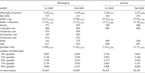
Table 1 provides descriptive statistics for the Washington and Arizona samples, broken down by first-child and second-child births. Any mother with missing data items in either of her two births (for the variables summarized in Table 1) was dropped from the sample. The resulting samples used for esti-mation consist of 45,067 Washington mothers (90,134 births)
Table 1. Descriptive statistics, Washington and Arizona birth panels
Washington Arizona
Variable 1st child 2nd child 1st child 2nd child
Birthweight (in grams) 3,442(523) 3,530(536) 3,339(517) 3,427(505)
Male child .515 .511 .520 .516
Mother’s age 25.27(5.25) 27.89(5.35) 25.23(5.26) 27.85(5.36)
Mother’s education 13.52(2.32) 13.72(2.21) 13.21(2.68) 13.39(2.61)
Married .751 .853 .780 .886
No prenatal care .004 .003 .005 .006
1st-trimester care .879 .895
2nd-trimester care .107 .093
3rd-trimester care .014 .012
Smoke .143 .132 .049 .044
Drink .017 .014 .009 .007
# prenatal visits 12.06(3.53) 11.63(3.25) 11.83(3.59) 11.73(3.55)
Quantiles of birthweight:
10% quantile 2,807 2,892 2,750 2,863
25% quantile 3,146 3,220 3,061 3,146
50% quantile 3,458 3,543 3,373 3,445
75% quantile 3,770 3,855 3,685 3,742
90% quantile 4,060 4,167 3,968 4,040
# of observations 45,067 45,067 56,201 56,201
and 56,201 Arizona mothers (112,402 births). Sample averages are reported for all variables, as well as standard deviations for the nonindicator variables. The “Smoke” (“Drink”) variable is equal to 1 if the mother reported smoking (drinking alcohol) during pregnancy. Although alcohol consumption during preg-nancy is known to be severely underreported, the “Drink” vari-able is included in the regressions as it may be useful as a proxy for other unobservables. For Washington, the four prenatal-care categories (“No prenatal prenatal-care,” “1st-trimester prenatal-care,” “2nd-trimester care,” “3rd-“2nd-trimester care”) were constructed on the basis of the reported month of the first prenatal-care visit. Un-fortunately, the month of first prenatal-care visit is not reported in the Arizona data until 1997. As a result, only the number of prenatal visits and an indicator variable for “no prenatal care” (equal to 1 if there are no prenatal visits) are summarized in Ta-ble 1 and used in the empirical analysis of Section 4. The other variables are self-explanatory.
The descriptive statistics in Table 1 indicate that average birthweight increases by 88 grams at the second birth for both Washington mothers and Arizona mothers. For their second birth, women are less likely to smoke and drink and more likely to be married, have a male child, and have a first-trimester prenatal-care visit. Based on the summary statistics, the two samples of mothers are quite similar. On average, Arizona mothers are slightly less educated and have higher birthweight babies. The largest difference between the two samples appears to be the level of smoking: Washington mothers report smoking in 13.7% of pregnancies (close to the national average during this time period), whereas only 4.7% of Arizona mothers re-port smoking. These smoking percentages are below the overall smoking percentages for pregnant women in these two states during the periods of interest (8.9% in Arizona and 18.4% in Washington), indicating that the matching algorithms result in subsamples that overrepresent nonsmokers. For instance, un-married Arizona mothers (for whom the smoking percentage is
12.7%) are far more likely to have father’s date-of-birth miss-ing from the data (45.9% of the time, as compared to 1.1% for married mothers) and, therefore, not included in the matched sample. The reported rate of drinking during pregnancy is also lower in Arizona than Washington; these reported percentages are also lower than the overall percentages for pregnant women in the two states (2.7% in Washington, 1.4% in Arizona).
Table 1 also provides the (unconditional) 10%/25%/50%/ 75%/90% quantiles for first and second births in Washington and Arizona. These quantiles indicate fairly symmetric birth-weight distributions, with the median quite close to the mean, the 25% and 75% quantiles roughly equidistant from the me-dian, and the 10% and 90% quantiles roughly equidistant from the median. For both states, there is a positive shift in the entire birthweight distribution from first to second births. The shift is largest in magnitude at the 90% quantile (107 grams) for Wash-ington births and at the 10% quantile (113 grams) for Arizona births. Finally, we note that the LBW cutoff of 2,500 grams corresponds to the 3–5% quantiles of the unconditional birth-weight distributions, whereas the HBW cutoff of 4,000 grams corresponds to the 85–92% quantiles of the unconditional dis-tributions.
4. RESULTS
Regression results for the two maternally linked datasets are provided in Section 4.1, within the strict-exogeneity framework introduced in Section 2. A straightforward approach to hypoth-esis testing is provided in Section 4.2. Section 4.3 provides dis-cussion related to possible violations of strict exogeneity (e.g., feedback effects or mismeasured variables).
4.1 Regression Results
In the interest of space, the full set of numerical results (tables) and a detailed discussion are provided only for the
Washington data (Sec. 4.1.1). The Arizona results are reported in a graphical format comparable to the Washington results (Sec. 4.1.3), but the detailed tables have been omitted and the discussion is limited to comparisons with the Washington re-sults. (Complete tables are available upon request from the au-thors.)
4.1.1 Washington Data. The tables report estimates for the quantiles τ ∈ {.10, .25, .50, .75, .90} (along with least squares estimates for comparison), although the figures pre-sented in this section consider marginal effects at 2% intervals (specifically,τ ∈ {.04, .06, . . . , .94, .96}). Throughout this sec-tion, the dependent variable of interest is birthweight (measured in grams). To have a relevant comparison for the panel-data re-sults, cross-sectional results (without incorporating the corre-lated random effects) are also reported. For the cross-sectional results, the panel structure of the data is only used for comput-ing standard errors. Since each mother appears twice in the data, the pair-sampling bootstrap described at the end of Section 2.2 is used.
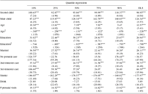
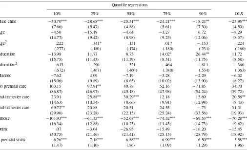
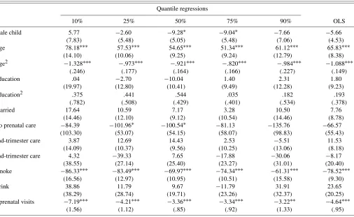
Tables 2 and 3 report the cross-sectional results and panel-data results, respectively. The model specification includes the variables summarized in Table 1, along with an indicator vari-able for the second child, quadratic varivari-ables for both mother’s age and education, and a full set of year-of-birth dummy vari-ables. For the prenatal-care variables, the omitted category cor-responds to first-trimester prenatal care, so the estimates for the
other three prenatal-care variables (“No prenatal care,” “2nd-trimester care,” and “3rd-“2nd-trimester care”) should be interpreted as differences from first-trimester prenatal care. The effect of prenatal care will therefore be captured by (1) the trimester of the first prenatal visit (if any) and (2) the number of prenatal visits (if any).
It should be pointed out that interpreting the effect of any prenatal-care variable is a bit difficult since theobserved prena-tal care proxies for bothintendedprenatal care and pregnancy problems. For instance, if two mothers have identical intentions (at the beginning of pregnancy) with respect to prenatal-care visits, the mother that experiences problems early in her preg-nancy would be more likely to have an earlier first prenatal-care visit and to have more prenatal-prenatal-care visits overall. The es-timated effects of the prenatal-care variables, therefore, may reflect the combined effects of intended care and pregnancy complications. This idea has been independently investigated by Conway and Deb (2005), who (1) found that bimodal resid-uals result from a standard 2SLS regression of birthweight and (2) used a two-class mixture model to explicitly allow for a dif-ference between “normal” and “complicated” pregnancies. The estimates for the no-prenatal-care indicator variable in both Ta-bles 2 and 3, which are significantly negative at the 10% quan-tile and significantlypositiveat the 90% quantile, illustrate this point. A possible explanation for the dramatic difference at the two ends of the distribution is that lack of prenatal care is more
Table 2. Cross-sectional estimation results, Washington data
Quantile regressions
10% 25% 50% 75% 90% OLS
Second child 100.65∗∗∗ 92.87∗∗∗ 93.86∗∗∗ 99.99∗∗∗ 110.37∗∗∗ 98.95∗∗∗
(7.24) (4.96) (4.40) (4.89) (6.84) (4.04)
Male child 87.22∗∗∗ 115.87∗∗∗ 128.34∗∗∗ 142.70∗∗∗ 160.83∗∗∗ 124.34∗∗∗
(6.25) (4.33) (3.85) (4.25) (5.65) (3.57)
Age 19.30∗∗∗ 13.81∗∗∗ 7.39∗∗ 7.92∗∗ 5.47 12.57∗∗∗
(6.35) (4.02) (3.58) (3.93) (5.17) (3.41)
Age2 −.385∗∗∗ −.258∗∗∗ −.131∗∗ −.122∗ −.070 −.228∗∗∗
(.115) (.070) (.064) (.070) (.091) (.061)
Education 31.02∗∗ 22.46∗∗ 30.23∗∗∗ 28.81∗∗∗ 23.87∗∗ 26.94∗∗∗
(14.32) (8.80) (7.70) (6.71) (10.45) (7.16)
Education2 −.744 −.603∗ −.927∗∗∗ −.987∗∗∗ −.793∗∗ −.789∗∗∗
(.525) (.324) (.285) (.250) (.388) (.264)
Married 36.58∗∗∗ 27.52∗∗∗ 26.74∗∗∗ 22.41∗∗∗ 16.20∗ 28.11∗∗∗
(10.22) (7.61) (6.03) (6.91) (9.19) (6.23)
No prenatal care −324.75∗ −22.76 −36.05 15.54 176.44∗∗ −34.57
(177.34) (55.29) (41.13) (44.24) (74.27) (47.90)
2nd-trimester care 37.34∗∗∗ 27.93∗∗∗ 24.72∗∗∗ 31.58∗∗∗ 37.96∗∗∗ 38.73∗∗∗
(11.86) (8.41) (7.00) (8.27) (10.43) (6.48)
3rd-trimester care 106.60∗∗∗ 59.36∗∗∗ 37.26∗ 26.07 24.40 66.39∗∗∗
(30.75) (20.43) (19.79) (18.81) (23.84) (15.96)
Smoke −186.05∗∗∗ −182.29∗∗∗ −178.57∗∗∗ −176.05∗∗∗ −160.02∗∗∗ −177.97∗∗∗
(11.40) (7.64) (6.23) (7.51) (9.92) (6.16)
Drink −21.80 −20.08 −7.27 −15.01 17.03 3.89
(28.14) (22.67) (16.10) (20.00) (26.55) (16.47)
# prenatal visits 19.33∗∗∗ 16.52∗∗∗ 15.11∗∗∗ 14.82∗∗∗ 13.92∗∗∗ 18.46∗∗∗
(1.35) (.89) (.76) (.82) (1.10) (.85)
NOTE: The dependent variable is birthweight (in grams). Bootstrapped standard errors in parentheses, using bootstrap sample size of 20,000 (10,000 pairs) and 1,000 bootstrap replications. Year dummies were included in all regressions.∗: significant at 10% level (2-sided);∗∗: 5% level;∗∗∗: 1% level.
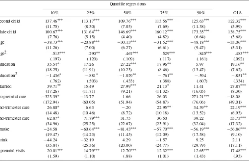
Table 3. Panel-data estimation results (βτ), Washington data
Quantile regressions
10% 25% 50% 75% 90% OLS
Second child 137.46∗∗∗ 113.17∗∗∗ 109.76∗∗∗ 113.56∗∗∗ 125.63∗∗∗ 122.32∗∗∗
(11.75) (8.30) (7.03) (7.69) (11.38) (5.99)
Male child 100.67∗∗∗ 131.64∗∗∗ 146.69∗∗∗ 160.12∗∗∗ 173.35∗∗∗ 138.75∗∗∗
(7.76) (5.15) (4.40) (4.82) (6.64) (3.68)
Age −38.73∗∗∗ −20.88∗∗∗ −30.13∗∗∗ −31.52∗∗∗ −48.18∗∗∗ −33.06∗∗∗
(11.26) (7.00) (6.27) (6.61) (9.47) (5.31)
Age2 .515∗∗∗ .290∗∗ .467∗∗∗ .529∗∗∗ .845∗∗∗ .483∗∗∗
(.197) (.120) (.109) (.117) (.161) (.092)
Education 35.54∗ 17.26 27.22∗∗∗ 17.96∗∗ 5.97 19.16∗∗
(18.25) (11.91) (10.23) (8.46) (13.47) (7.62)
Education2 −1.436∗ −.881∗ −1.029∗∗ −.761∗∗ −.594 −.851∗∗
(.762) (.503) (.433) (.388) (.607) (.334)
Married 39.71∗∗ 15.49 27.99∗∗∗ 21.13∗ 11.41 27.87∗∗∗
(17.26) (11.71) (9.21) (11.32) (16.05) (8.30)
No prenatal care −323.39∗ −13.77 1.66 26.03 271.21∗∗∗ −18.08
(172.94) (60.05) (51.94) (54.87) (76.06) (49.01)
2nd-trimester care 26.80∗ 6.63 −.20 22.95∗∗ 34.39∗∗ 22.19∗∗∗
(14.48) (10.46) (8.72) (10.18) (13.52) (6.93)
3nd-trimester care 62.87∗ 71.79∗∗∗ 31.75 30.50 39.22 55.73∗∗∗
(34.96) (25.25) (22.67) (23.91) (32.04) (17.32)
Smoke −24.58 −60.64∗∗∗ −81.43∗∗∗ −57.70∗∗∗ −56.19∗∗∗ −56.86∗∗∗
(19.47) (14.23) (11.45) (12.09) (17.58) (9.10)
Drink −44.24 −32.19 4.29 −1.57 9.25 2.11
(35.84) (25.36) (20.00) (24.77) (29.79) (17.11)
# prenatal visits 20.01∗∗∗ 14.79∗∗∗ 12.70∗∗∗ 12.32∗∗∗ 12.65∗∗∗ 17.48∗∗∗
(1.59) (1.10) (.88) (1.01) (1.43) (.93)
NOTE: The dependent variable is birthweight (in grams). Bootstrapped standard errors in parentheses, using bootstrap sample size of 20,000 (10,000 pairs) and 1,000 bootstrap replications. Year dummies were included in all regressions.∗: significant at 10% level (2-sided);∗∗: 5% level;∗∗∗: 1% level.
likely to proxy for lack of intended care at the lowest quan-tiles and more likely to proxy for a problem-free pregnancy at the highest quantiles. Alternatively, the positive effect found at higher quantiles could still be consistent with a lack of intended care since HBW outcomes have previously been associated with poor prenatal care and disadvantaged mothers. (Unfortu-nately, the leading indicators of HBW outcomes are mother’s weight prior to pregnancy and weight gain during pregnancy. Neither of these items is available in the datasets, forcing us to focus less on the effects of birth inputs on HBW outcomes.) At the intermediate quantiles, the effect of the no-prenatal-care in-dicator is found to be statistically insignificant in both the cross-sectional and the panel results.
Overall, the cross-sectional results in Table 2 are very simi-lar to those found in previous studies using federal natality data (Abrevaya 2001; Koenker and Hallock 2001). For the panel-data results in Table 3, unobserved heterogeneity is modeled as in Section 2.2 [see (16) and (17)]. For the pooled quantile regressions, Table 3 reports the estimates of the marginal ef-fectsβτ. The estimates of the parametersλ1τ andλ2τare reported
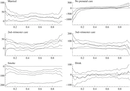
in Appendix B (Tables 5 and 6); these estimates measure the ex-tent of the cross-sectional bias (through the relationship of the unobserved heterogeneity with the observables). To provide a more complete view of the variables’ effects on birthweights and to allow an easy comparison with the cross-sectional es-timates, Figures 1 and 2 plot the estimated effects from both the panel and the cross section. For these figures, the quantile
regressions were estimated at 2% intervals, from the 4% quan-tile through the 96% quanquan-tile (inclusively). The panel-data es-timates are represented with a solid line, and the 90% confi-dence intervals (bootstrap percentile intervals) for these esti-mates are represented with dotted lines. The cross-sectional es-timates, computed at the same quantiles, are represented with a dashed line. [To avoid cluttering the figures, confidence inter-vals for the cross-sectional results (which can be inferred from Table 2) are not reported.] Since both age and education have quadratic terms in the model specification, the marginal-effect plots for age and education are based upon estimates evaluated at specific values for the two variables (25 years old for age and 12 years for education level).
The estimated effects of the various variables, as presented in Tables 2 and 3 and Figures 1 and 2, are discussed in more detailed below:
Second child: Birthweights are uniformly larger for second children at all quantiles, for both the cross-sectional and panel estimates. The panel estimates of the second-child effect are somewhat larger than the cross-sectional esti-mates, with the largest effects at the lowest quantiles (e.g., 137 grams at the 10% quantile).
Male child: It is well known that, on average, male babies weigh more at birth than female babies. The quantile esti-mates indicate that the positive male-child effect on weight is present at all quantiles of the conditional birth-weight distribution. The magnitude of the effect increases
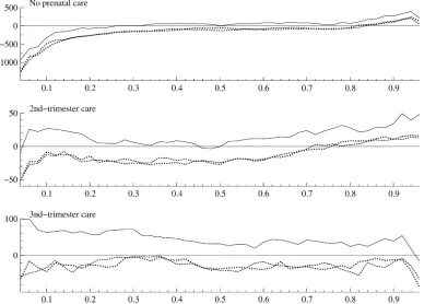
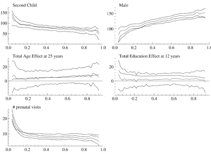
Figure 1. Part 1 of the estimated marginal effects on the conditional quantiles for Washington births. The dependent variable is birthweight (in grams). The solid line indicates the panel-data estimates, the dotted lines are 90% confidence bands for the panel-data estimates, and the dashed line indicates the cross-sectional estimates.
Figure 2. Part 2 of the estimated marginal effects on the conditional quantiles for Washington births. The dependent variable is birthweight (in grams). The solid line indicates the panel-data estimates, the dotted lines are 90% confidence bands for the panel-data estimates, and the dashed line indicates the cross-sectional estimates.
when one moves from lower quantiles to higher quantiles, with the panel estimates indicating a slightly higher effect (10–20 grams) than the cross-sectional estimates. Age and education: Figure 1 shows the estimated (one-year)
effects of age and education, evaluated at 25 years of age and 12 years of education, respectively. For age, both the cross-sectional and panel estimates are very close to zero in magnitude (and statistically insignificant at a 5% level for all quantiles). For education, the cross-sectional es-timates are positive across the quantiles and statistically significant (at a 5% level) except at quantiles above 80%. In contrast, the panel estimates are statistically insignifi-cant across all quantiles. This difference could be due to two factors: (1) the amount of within-mother variation in education is quite small, with the average change in ed-ucation for the sample being about .2 years, and (2) the level of education may be related to the mother-specific unobservable. For the latter factor, years of schooling is likely positively related tocm, which would imply an
up-ward bias in the cross-sectional estimates that is consis-tent with Figure 1. The issue of education being poten-tially mismeasured is briefly discussed in Section 4.3.2. Results for other age and education levels are reported in Abrevaya and Dahl (2006).
Marital status: The estimated positive effects of marriage on birthweight are quite similar for the cross-sectional and panel specifications, in the 20–50-gram range over the quantiles considered. One should be cautious about in-terpreting the cross-sectional marriage estimates as causal because marital status is an explanatory variable that a pri-ori would appear to serve as a proxy for mother-specific unobservables (i.e., marital status positively correlated with cm). The panel estimates are slightly lower than
the cross-sectional estimates in the lower quantiles (un-til around the 40% quan(un-tile), suggesting that this might be a factor in the lower quantiles. Somewhat surprisingly, however, the panel estimates of the marriage effect remain positive throughout the range of quantiles and signifi-cantly so (at the 10% level) at nearly all the quantiles be-low 80%. On the whole, the estimates are consistent with a situation in which marriage provides the birth mother with support (financial support, emotional support, and so on) that would lead to a more favorable birth outcome. Prenatal-care visits: Lack of prenatal care is found to have
significant negative effects at the lower quantiles and sig-nificant positive effects at the upper quantiles. The es-timated effects are similar for both the cross-sectional and panel regressions. As discussed previously, a logi-cal explanation is that the “No prenatal care” indicator variable may proxy for poor care at lower quantiles, but for problem-free pregnancies at upper quantiles. For the third-trimester-care indicator variable, the cross-sectional and panel estimates are also similar, indicating positive effects (as compared to first-trimester care) which be-come less statistically significant at higher quantiles. For the indicator variables, the largest difference between the cross-sectional and panel results shows up in the second-trimester-care variable; the cross-sectional estimates are statistically significant at all quantiles and range from 25
grams to 50 grams, whereas the panel estimates are some-what lower (close to zero in intermediate quantiles) and only significantly positive at the highest quantiles. The effect of the number of prenatal visits is estimated to be significantly positive across all quantiles, with larger ef-fects found at lower quantiles and the efef-fects essentially “flattening out” (at around 14–15 grams per visit for the cross-sectional results and 12–13 grams per visit for the panel results). The estimated effects for the panel spec-ification exhibit a sharper decline, leading to lower esti-mates (roughly a 2-gram per-visit differential) than for the cross-sectional specification. This variable shows up sig-nificantly in theλ1τ andλ2τ estimates (see Tables 5 and 6), leading to the differences found and suggesting that the variable is related to the mother-specific unobservable. Smoking: The most dramatic differences between the
cross-sectional and panel results are the estimated effects of smoking. The cross-sectional results indicate that the negative effects of smoking are in the range of 150– 200 grams, with larger effects at lower quantiles. The panel estimates are still significantly negative at all but the lowest quantiles, but the estimated effects are much lower in magnitude (mostly in the 50–80-gram range be-tween the 20% and 80% quantiles). The omitted-variables explanation of this large difference would be that the smoking indicator in the cross-sectional specification is negatively related with the error disturbance in the birth-weight regression equation. Consistent with this expla-nation, the smoking coefficients in both λ1τ and λ2τ are found to be significantly negative across the quantiles (Ta-bles 5 and 6). The magnitudes of the panel estimates are also significantly lower than those found in previ-ous work, including quasi-experimental estimates based upon cigarette-tax changes (e.g., Evans and Ringel 1999; Lien and Evans 2005) and experimental estimates (e.g., Permutt and Hebel 1989). These studies have estimated causal (IV) effects of smoking on birthweight that are not statistically different from the OLS estimates; these es-timates have relatively large standard errors (due to the sources of variation exploited) and, in some cases, are evenlargerin magnitude than the OLS estimates. We be-lieve that our panel estimates are quite credible given the compelling nature of the omitted-variables explanation in this context. We note, however, that our results do not directly contradict those found by instrumental-variables methods. First, the IV estimates are quite imprecise (large standard errors), so our estimates would also fall within reasonable confidence intervals for these previous studies. Second, the panel estimates are identified from mothers who change their smoking status for any reason, whereas the IV estimates are identified from mothers who change their smoking status in response to a specific treatment (e.g., prenatal counseling or cigarette-tax increases); be-cause these subpopulations are different, the underlying treatment effects could themselves also be different. Fi-nally, we point out that misclassification of smoking sta-tus could explain part of the difference found here because the effect of misclassification is more severe in the panel-data case (see, e.g., Freeman 1984; Jakubson 1986). This possibility is further discussed in Section 4.3.2.
Alcohol consumption: In contrast to the smoking results, the estimated effects of alcohol consumption are quite similar for the cross-sectional and panel specifications. Drinking is estimated to have significant negative effects at lower quantiles (below about the 20% quantile), with the mag-nitudes of the effects ranging between about 40 and 80 grams. Of course, very few mothers actually report alco-hol consumption during pregnancy (only about 1.5% in our sample). The lack of strong statistical evidence re-garding the effects of drinking could stem from the low variation in the indicator variable and the probable large rates of misclassification.
4.1.2 “Overcontrolling” and Interpretation of Estimates. If one is interested in the “structural” estimates related to pre-natal care and smoking, it is not obvious which variables should be included in the regression specification. In particular, the es-timates presented above are identified from within-mother vari-ation (rather than varivari-ation induced by a specific policy), but we would like to be able to offer an interpretation of the estimates relevant to potential policy impacts. What would be the effect of a policy that increased the likelihood of a first-trimester prena-tal visit? What would be the effect of a policy that reduced the likelihood of prenatal smoking? Related to these two questions, there are potential concerns with the specification used above, which includes variables for prenatal-care initiation, number of prenatal visits, and smoking status. If earlier prenatal-care initi-ation (e.g., a first-trimester visit) has the “mechanical” effect of increasing the number of prenatal-care visits, inclusion of the number of visits as a covariate effectively “overcontrols” for the effect of early prenatal-care initiation. Similarly, if prenatal
care affects birthweight only through its effect on smoking ini-tiation, inclusion of smoking status as a covariate could also be an “overcontrolling” factor.
To empirically assess the possible importance of “overcon-trolling,” we reran the Washington regressions under two al-ternative specifications: (1) original specification with number of prenatal visits dropped, and (2) original specification with number of prenatal visits, smoking status, and drinking sta-tus dropped. Figure 3 reports the estimates on the prenatal-care-initiation categorical variables for these two specifications along with the original specification. Dropping the number of prenatal visits from the specification has important con-sequences. For each of the three variables (which are inter-preted as differences from first-trimester care), there is a sig-nificant drop in the coefficient estimates across the quantiles. The second-trimester estimate goes from being positive (and statistically insignificant) at most quantiles to being negative and statistically significant (at a 10% level) at all quantiles be-low 60%. The no-prenatal-care variable also becomes negative and statistically significant (at a 10% level) at all quantiles be-low 60%. (Note the difference in scale on theyaxes for the three variables.) The third-trimester estimate goes from being signif-icantly positive at most quantiles to being negative, but statisti-cally insignificant, at most quantiles. Overall, if one views first-trimester prenatal care as mechanically increasing the number of prenatal-care visits, the estimates from Figure 3 indicate that the structural effect of increasing early prenatal-care initiation would be to increase birthweight at lower quantiles (with small effects of about 20 grams for transitions from second-trimester care to first-trimester care and much larger effects for transi-tions from no prenatal care to first-trimester care). We also note
Figure 3. Results for initial-prenatal-visit variables under different specifications (Washington data). The solid line corresponds to the full specification, the dotted line to the specification in which “# of prenatal visits” is dropped, and the dashed line to the specification in which “# of prenatal visits,” “Smoke,” and “Drink” are dropped. The omitted category is first-trimester care.
that the estimates on the other variables (those not shown in Fig. 3) remain essentially unchanged when number of visits is dropped from the specification.
When smoking status and drinking status are also dropped from the specification, there is essentially no change in the prenatal-care-initiation estimates shown in Figure 3 (the com-parison between the dotted and dashed lines). This suggests that the inclusion of smoking status in the original specification (and also in the one dropping number of visits) did not have an im-pact on the estimated effect of the timing of prenatal-care ini-tiation. Alternatively, in thinking of other variables as possibly “overcontrolling” for smoking status, we tried several cations in which other covariates were dropped from specifi-cations in which smoking status remained. For these specifica-tions, we found estimated smoking effects that were extremely similar to those reported in Figure 1. These results make us more comfortable about interpreting the original smoking esti-mates (Fig. 1) as structural effects upon the conditional quantile distribution.
4.1.3 Arizona Data. Figures 4 and 5 plot the estimated quantile effects (4% through 96% quantiles, inclusively) for the Arizona maternally linked sample. The same model spec-ification discussed previously was used, except that indicator variables for second-trimester and third-trimester prenatal care were not included. The figures are comparable to Figures 1 and 2 for the Washington data, with the age effect reported at 25 years and the education effect at 12 years.
Overall, there is a remarkable similarity between the results for the two samples. The common findings for the two samples include the following:
• There is a significant positive effect of the second child across all quantiles (50–125 grams in the Arizona panel estimates).
• The positive birthweight effect of a male child increases from lower to higher quantiles.
• Despite a positive estimated cross-sectional effect of edu-cation at lower quantiles, the panel estimates indicate no significant education effect.
• The effect of the number of prenatal visits is highest at lower quantiles, with the effect flattening out at higher quantiles. For both Washington and Arizona, the cross-sectional estimate of the effect is lower at lower quantiles and higher at higher quantiles.
• The magnitude of the negative smoking effect is signifi-cantly lower for the panel estimates (ranging between 40 and 80 grams for Arizona) than for the cross-sectional es-timates.
Some differences between the results for the two samples are also worth noting:
• Although the cross-sectional estimates of the marriage ef-fect are still significantly positive (p-values lower than .10 throughout the range of quantiles), the panel-data es-timates indicate no statistically significant effect of mar-riage for Arizona mothers. The likely explanation of this
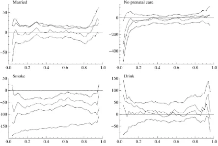
Figure 4. Part 1 of the estimated marginal effects on the conditional quantiles for Arizona births. The dependent variable is birthweight (in grams). The solid line indicates the panel-data estimates, the dotted lines are 90% confidence bands for the panel-data estimates, and the dashed line indicates the cross-sectional estimates.
Figure 5. Part 2 of the estimated marginal effects on the conditional quantiles for Arizona births. The dependent variable is birthweight (in grams). The solid line indicates the panel-data estimates, the dotted lines are 90% confidence bands for the panel-data estimates, and the dashed line indicates the cross-sectional estimates.
finding is that the father’s date of birth is required to match for both births of an Arizona mother (see Sec. 3), mean-ing that the father is the same even if marital status differs across the births. For the Washington sample, a change in marital status might also be related to a change in father. • Because of the lack of indicator variables for
second-trimester and third-second-trimester care, the estimated effects of the no-care indicator variable and the number of prenatal visits are slightly different. The magnitude of the quan-tile effects for number of prenatal visits is roughly 50% lower for the Arizona sample, although the shape of the quantile-effect curve is extremely similar. The shape of the no-prenatal-care effect is also very similar to that of Wash-ington, but the estimated panel effects are not significantly different from zero at any of the quantiles.
4.2 Hypothesis Testing
In this section, we discuss the results of several hypothe-sis tests that were used to test the model specification and/or the significance of differences across the estimates at different quantiles. The minimum-distance (MD) framework of Buchin-sky (1998) is used (and extended to the panel-data case) to test various (linear) restrictions placed on the parameters in the es-timated models.
4.2.1 Minimum-Distance Testing Framework. Let p de-note the number of different quantiles at which the model is estimated, withτ1, . . . , τp denoting the quantiles. For a given
quantileτ, individual elements of the parameter vectorsβτ,λ1τ,
and λ2τ [recall the model in (16) and (17)] are referenced by subscripts as follows:
βτ=(βτ1, . . . , βτL)′,
λ1τ=(λ1τ1, . . . , λ1τK)′, λ2τ=(λ2τ1, . . . , λ2τK)′,
whereKis the number of variables inxm1andxm2. For gener-ality,βτ hasL≥K elements, to allow for additional variables
(e.g., time-invariant regressors) that may not appear in theλ es-timates. Then, for a given quantileτ, the full parameter vector is denoted
γτ≡(φτ1, βτ0, βτ′, λ1
′
τ, λ2τ′)′, (19)
whereβτ0≡φτ2−φτ1. The (stacked) parameter vector for all of
the estimated quantiles is denoted
γ≡γτ′
1, γ ′
τ2, . . . , γ ′
τp
′
(20)
and has dimension p(2K+L+2)×1. Further, letγ denote the estimator ofγ, and defineAto be the estimated variance– covariance matrix (obtained via the bootstrap) ofγ.
In the MD framework, the “restricted” parameter estimator is defined as
γR=arg min
γR∈
(γ−RγR)′A−1(γ−RγR), (21) whereRis a restriction matrix that will depend on the type of restrictions imposed. Since only linear restrictions are consid-ered,γRcan be written explicitly as
γR=(R′A−1R)−1(R′A−1γ ). (22)
The asymptotic variance ofγRis given by
var(γR)=(R′A−1R)−1. (23) For the purposes of hypothesis testing, note that under the null hypothesis that the restrictions are true (i.e.,H0:γ=RγR), the following MD test statistic has a limiting chi-square distribu-tion:
(γ−RγR)′A−1(γ−RγR)−→d
H0
χM2, (24) where M is the number of restrictions [i.e., M =rows(R)− columns(R)]. Appendix A provides specific details on the ap-propriate choice ofRandMfor each of the tests described be-low.
4.2.2 Test Results. Using the MD testing framework, the following hypothesis tests were conducted:
Test of correlated random effects: To determine whether a “pure” random-effects specification (in whichcm is
un-correlated with xm) would be rejected for a given
quan-tileτ, the null hypothesisH0:λ1τ=λ2τ=0 is tested. For
the quantilesτ ∈ {.10, .25, .50, .75, .90}, the null hypoth-esis is overwhelmingly rejected withp-values extremely close to zero.
Test of the equality of the “effect vector” across quantiles: This test considers whether there areanystatistically sig-nificant differences in theβτ estimates across two
differ-ent quantiles. For the panel specifications, we conducted this test for each pairwise combination of quantiles from the set {.10, .25, .50, .75, .90}. For Washington, the p -values (all below 2%) indicate very significant differences across the quantiles. For Arizona, there are significant dif-ferences between the lowest quantiles (10% and 25%) and other quantiles; however, thep-values for the 50%/90% and the 75%/90% comparisons do not indicate a statisti-cally significant difference in theβτ estimates.
Test of the equality of individual variables’ effects across quantiles:For a given variable (e.g., marital status), this test checks whether the estimated effects at different quantiles are significantly different. The set of differ-ent quantiles considered is the same as that used in Ta-bles 2 and 3. For the marriage indicator, for instance, the null hypothesis would be H0:βτmarried=.10 =βτmarried=.25 =
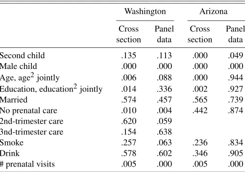
βτmarried=.50 =βτmarried=.75 =βτmarried=.90 . Since both age and edu-cation enter into the model specifiedu-cation in two terms (a linear term and a quadratic term), the appropriate tests for these two variables are joint tests of equality. The test results (p-values) for all of the variables, in both the cross-sectional and the panel specifications, are reported in Table 4 for Washington and Arizona. The results are very much in line with the quantile-estimate graphs in Figures 1 and 2 and Figures 4 and 5. Two variables (male-child indicator and number of prenatal visits) vary sig-nificantly across the quantiles for both the cross-sectional and panel specifications. The effect of the no-prenatal-care indicator also varies significantly (p-value of .010 in the cross section and .004 in the panel) for the Wash-ington sample. On the other hand, there is no statistical evidence that the effects of marital status or drinking vary over quantiles in either specification. The cross-sectional
Table 4. Tests of marginal-effect equality across quantiles
Washington Arizona
Cross Panel Cross Panel section data section data
Second child .135 .113 .000 .049 Male child .000 .000 .000 .000 Age, age2jointly .006 .088 .000 .944 Education, education2jointly .014 .336 .002 .927
Married .574 .457 .565 .739
No prenatal care .010 .004 .442 .874 2nd-trimester care .620 .059
3nd-trimester care .154 .638
Smoke .257 .063 .236 .834
Drink .578 .602 .346 .905
# prenatal visits .005 .000 .005 .000
NOTE: For each covariate,p-values based upon cross-sectional and panel-data estimates are reported for the null hypothesis of equality of marginal effects for the five quantiles .10, .25, .50, .75, and .90. Results are based upon 1,000 bootstrap replications.
estimated effects of both age and education vary signif-icantly across quantiles, whereas the panel estimated ef-fects do not. For the smoking-indicator variable, the p -value for the Washington cross-sectional results is quite high (.396), whereas thep-value (.063) for the panel spec-ification suggests a more significant difference in the esti-mated effects across quantiles. Finally, it should be noted that the choice of the quantile set{.10, .25, .50, .75, .90} is admittedly arbitrary, following what has become the convention for quantile regression.
4.3 Endogeneity Issues
In this section, we consider the sensitivity of the estimation results to possible sources of endogeneity. Note that the esti-mation method introduced in Section 2 (and discussed further in Sec. 5) is based upon the assumption of strict exogeneity and, in general, will be inconsistent when this assumption is violated. The two most important sources of endogeneity in the current application are (1) a “feedback effect” by which the first-birth outcome (birthweight) influences second-birth ex-planatory variables (e.g., a low-birthweight first-birth outcome causing a mother to quit smoking for the second birth), and (2) mismeasured explanatory variables.
4.3.1 Feedback or Dynamic Effects. The issue of feed-back effects is discussed at length in Abrevaya (2006) in the context of a conditional-expectation model, where instrumental-variables methods (using lagged birthweights as instruments) can be utilized. Unfortunately, there is no obvious analogue to instrumental variables in the conditional-quantile context. In-stead, to see if allowing for dynamic effects alters the panel-data estimates in an important way, we consider an augmented model specification in which lagged birthweight is included as an explanatory variable. Specifically, because data on two births per mother are available,ym1(first-birth birthweight) is included as a right-side variable for the second-birth equation. (Considering matched panel data with three births per mother reduces the sample size to an extent that makes all of the es-timates imprecise.) Only a single coefficient for ym1 in the