POINT-BASED VERSUS PLANE-BASED SELF-CALIBRATION OF STATIC
TERRESTRIAL LASER SCANNERS
J.C.K. Chowa*, D.D. Lichtia, and C. Glennieb
a
Department of Geomatics Engineering, University of Calgary, 2500 University Dr NW, Calgary, Alberta, T2N1N4 Canada - (jckchow and ddlichti)@ucalgary.ca
b
Department of Civil & Environmental Engineering, University of Houston, 3605 Cullen Blvd, Houston, Texas, 77204-5059, United States of America – [email protected]
Commission V, WG V/3
KEY WORDS: Terrestrial, Laser scanning, LIDAR, Calibration, Modelling, Precision, Point Cloud, Analysis
ABSTRACT:
Systematic trends are apparent when studying the self-calibration residuals of many modern static terrestrial laser scanners. Since the operation of terrestrial laser scanners is comparable to an efficient robotic total station, the sensor modelling parameters are developed in the spherical coordinate system where the raw observables of the scanner are range, horizontal angle, and vertical angle. Sensor calibration parameters are already well established for both hybrid and panoramic type laser scanners through the signalized target-based self-calibration method. In this paper, a less labour-intensive and more efficient planar-feature based terrestrial laser scanner self-calibration method, which is more suitable for in-situ self-calibration, is presented. Through simulation it will be demonstrated that the point-based self-calibration and plane-based self-calibration shares many common characteristics. Plane-based self-calibration results from real data captured with the panoramic type Leica HDS6100 and hybrid type Trimble GS200 scanner are also presented to show the practicality of the proposed method and as a comparison to the point-based self-calibration.
* Corresponding author.
1. INTRODUCTION
The importance of sensor modelling for static terrestrial laser scanning (TLS) instruments has been gaining recognition over the years (Amiri Parian and Gruen, 2005; Schneider and Schwalbe, 2008; Reshetyuk, 2009; González-Aguilera et al., 2011). To ensure optimum performance of a TLS instrument all systematic errors of the 3D imaging sensor need to be adequately modelled/eliminated. This modelling includes both calibration of the individual components and the estimation of misalignment between them. Previous studies have shown that a suitable method of calibration is to analyse the residuals in range, horizontal angle, and vertical angle and model systematic trends in the spherical coordinate system (Lichti, 2007; Chow et al., 2010a). In Lichti (2007), a set of sensor modelling parameters suitable for most pulse-based and phase-based laser scanners having either a hybrid or panoramic architecture was developed for a point-based self-calibration. The geometric quality of the 3D coordinates obtained from the TLS sensor can be improved through the point-based self-calibration approach (Reshetyuk, 2006; Chow et al., 2010b).
One of the biggest drawbacks of point-based TLS self-calibration is that to ensure strong network geometry, a large quantity of signalized targets covering the entire field of view (FOV) of the scanner needs to be deployed (Lichti, 2010). Although low-cost paper targets can be utilized for this process (Chow et al., 2010a), this can still be time consuming, and depending on the scene certain areas (e.g. ceiling) may not be easily accessible (Reshetyuk, 2010). Alternatively, features such as planes can be used instead of signalized targets in the calibration routine. The concept of plane-based self-calibration for static TLS instruments have been reported in Gielsdorf et al. (2004), Bae and Lichti (2007), Dorninger et al. (2008), Molnár (2009), and Glennie and Lichti (2010). For mobile laser scanning systems a plane-based approach has been
used to model errors internal to the laser scanner and parameters relating multiple sensors such as the boresight angles (Skaloud and Lichti, 2006; Rieger et al., 2010).
In this paper, the point-based and plane-based TLS self-calibration methods for static scanners will be compared using both simulated and real data. In the simulation, the four most fundamental systematic errors: rangefinder offset, vertical circle index error, trunnion axis error, and collimation axis error are tested for both hybrid and panoramic type scanners. The issue of model identification and parameter correlation as stated in Lichti et al. (2011) will be addressed. Besides simulation, point clouds captured by a pulse-based hybrid type TLS instrument (Trimble GS200) and phase-based panoramic type TLS instrument (Leica HDS6100) will be used in both a point-based and plane-based self-calibration for comparison.
2. MATHEMATICAL MODEL
As in the point-based TLS self-calibration (Lichti, 2007), sensor modelling is carried out in the spherical coordinate system.
the Cartesian coordinates of point i in scanner space j; Δρ, Δθ, Δα are the additional systematic correction parameters for range, horizontal angle, and vertical angle, respectively.
When using planes as targets in the TLS self-calibration the observations from the scanner are constrained to lie on each plane through the point-on-plane-condition equation. Using the well-known Gauss-Helmert model (also known as combined model), the plane parameters, exterior orientation parameters (EOPs), and calibration parameters are solved simultaneously in a least-squares adjustment.
ij cj
k 0T j T
k M p P d
n (2)
where nk is the normal vector of plane k; Mj is the 3D rotation matrix defining the orientation of scanner j as a function of the Cardan angle sequence; pij is a vector that consists of xij, yij, zij; Pcj defines the 3D position of scanner j; dk is the orthogonal distance from the origin to plane k. Details on the solution of this model can be found in Förstner and Wrobel (2004).
3. SIMULATION RESULTS
In sections 3.1 and 3.2 the issue of model identification for panoramic and hybrid scanners, respectively, will be addressed by showing how systematic errors propagate into the residual plots in a plane-based TLS self-calibration. From Lichti et al., (2011) it has been shown that systematic errors are easier to identify and recover for panoramic scanners because they can observe vertical angles with a much wider range (180o <
range) than hybrid scanners (range≤ 180
o
). This greater range makes panoramic scanners more comparable to a theodolite observing directions in both telescope faces. For the simulations in this section a room with dimensions 14 m by 11 m by 3 m that consists of four walls (vertical planes), a ceiling, and a floor (horizontal planes) are simulated. In the point-based simulation each plane has 20 randomly distributed targets, and for the plane-based simulation there are 50 randomly distributed points on each of the six planes. All of the planes are assumed to be observable in the six scans captured from two nominal positions. The two positions are approximately 12 m apart horizontally and 60 cm apart vertically. At each position three levelled scans are captured with a heading that is separated by 120o to imitate the situation where the scanner is forced centred and rotated about the tribrach (Chow et al., 2010b; Lichti et al., 2011). In the simulation no noise was added to the EOPs of the scans. The noise level for the scanner’s range and angular observations are assumed to be 1 mm and 15”, respectively. These values are chosen based on the latest point-based self-calibration of the Leica HDS6100. The scanner is assumed to have unlimited horizontal and vertical FOV. The size of the laser footprint is not considered and it is assumed the scanner can observe equally accurate regardless of the incidence angle. Furthermore, the datum is defined simply by fixing the EOPs of the first scan.
3.1 Panoramic Type TLS Instruments
3.1.1 Panoramic - Rangefinder Offset: The rangefinder offset models the bias in distance measurements. This error could exist because of an unknown spatial offset between the laser firing point and the origin of the scanner coordinate system and/or electronic latency. It is usually modelled as a constant in the range measurements.
o
a
(3)Figure 1 below shows the propagation of an unmodelled 5 mm rangefinder offset into the residuals of a point-based TLS
self-calibration in the same simulated room under the same conditions as described in Section 3.
(a)
(b)
Figure 1: (a) Range residuals versus range plot in point-based self-calibration for panoramic scanners without systematic errors. (b) Unmodelled 5 mm rangefinder offset.
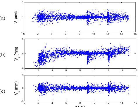
Figure 2 shows the effect of a 5 mm rangefinder bias in the plane-based TLS self-calibration. Instead of appearing as a near-linear trend as in the point-based TLS self-calibration the rangefinder offset appears as a quasi-logarithmic function. The reason for this can be explained by studying the incidence angle (Figure 3). When the laser is orthogonal to a plane, the range measurements are well constrained by the point-on-plane condition, hence a large deviation from zero can be perceived in the residuals when under the influence of ao. However, the angular observations, which are orthogonal to the range observation, are not restricted by the plane. As the laser incidence angle approaches 90o the angular observations become well controlled by the plane, but the range measurements can take on any value and still satisfy the point-on-plane condition, therefore the ρ residuals are near-zero even if an unmodelled ao exists. From this fact, it can be concluded that to analyse errors in the range direction, it is important to have observations with small incidence angles. On the contrary, for angular measurements it is important to have observations with large incidence angle based on the same principle. However, this might be a challenge in practice because it has been shown that points with a large incidence angle suffer from significantly lower signal-to-noise ratio for the distance measurements (Lichti, 2007; Soudarissanane et al., 2011). Future simulations will take into account the observation precision as a function of the incidence angle.
(a)
(b)
(c)
Figure 2: (a) Range residuals versus range plot in plane-based self-calibration for panoramic scanners without systematic errors. (b) Unmodelled 5 mm rangefinder offset. (c) After plane-based self-calibration.
Figure 3: Incidence angle of the laser as a function of range
3.1.2 Panoramic - Vertical Circle Index Error: A commonly encountered error in the vertical angle measurements is the vertical circle index error, which describes a constant offset between the scanner’s horizontal plane and the scanner’s zero elevation angle mark. This bias can be modelled as shown in Equation 4.
o
c
(4)The bias co (with a magnitude of 3’) propagates into the residuals of a point-based self-calibration as shown below in Figure 4. The residuals appear as two sinusoids both having a period of 360o but with opposite signs. The propagation of this error in a plane-based self-calibration appears as a single sinusoid with a period of 360o (Figure 5), which is consistent with the results from Lichti et al. (2011) where the vertical FOV of the scanner was restricted. Another important observation is the vast amount of α observations with near-zero residuals even when the systematic error is present. This can be attributed to the fact that a large number of observations are made with a near zero incidence angle, which provide minimal information for the calibration of angular errors.
(a)
(b)
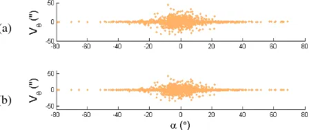
Figure 4: (a) Vertical angle residuals versus horizontal angle plot in point-based self-calibration for panoramic scanners without systematic errors. (b) Unmodelled 3’ vertical circle index error.
(a)
(b)
(c)
Figure 5: (a) Vertical angle residuals versus range horizontal angle in plane-based self-calibration for panoramic scanners without systematic errors. (b) Unmodelled 3’ vertical circle index error. (c) After plane-based self-calibration.
3.1.3 Panoramic - Trunnion Axis Error: The non-orthogonality between the trunnion axis and vertical axis of a TLS instrument is known as the trunnion axis error. It can be modelled with a tangent function of elevation angle. Equation 5 gives the error model used in the self-calibration.
b2tan
(5)
In the point-based self-calibration the tangent function is quite apparent even for a trunnion axis error of 1’, as demonstrated in Figure 6. However, in the plane-based self-calibration a larger error (e.g. 3’) is necessary before the trend becomes apparent in the residual plots as shown in Figure 7. Similar to the α residuals many near-zero residuals exist in the θ residuals of the plane-based self-calibration due to the small incidence angle.
(a)
(b)
Figure 6: (a) Horizontal angle residuals versus vertical angle plot in point-based self-calibration for panoramic scanners without systematic errors. (b) Unmodelled 1’ trunnion axis error.
(a)
(b)
(c)
(d)
Figure 7: (a) Horizontal angle residuals versus vertical angle plot in plane-based self-calibration for panoramic scanners without systematic errors. (b) Unmodelled 1’ trunnion axis error. (c) Unmodelled 3’ trunnion axis error. (d) After plane-based self-calibration.
3.1.4 Panoramic - Collimation Axis Error: The collimation axis error defines the non-orthogonality between the collimation axis and the trunnion axis. The commonly used mathematical model for self-calibration is given in Equation 6.
b1sec (6)
Figure 8 shows the effect of an unmodelled collimation axis error with a magnitude of 1’ in the point-based self-calibration. For panoramic scanners it causes the clusters of θ residuals belonging to the observations in front and behind the sensor to have a bias with the same magnitude but opposite signs. The effect of the same systematic error in the plane-based self-calibration has an odd-symmetric pattern that is similar to the point-based self-calibration (Figure 9).
Figure 8:Horizontal angle residuals versus vertical angle plot of unmodelled 1’ collimation axis error in point-based self-calibration for panoramic scanners.
(a)
(b)
Figure 9: (a) Unmodelled 1’ collimation axis error. (b) After plane-based self-calibration.
3.2 Hybrid Type TLS Instruments
3.2.1 Hybrid - Rangefinder Offset: From previous studies utilizing point-based self-calibration it has been demonstrated that a range bias propagates into the residuals in the same fashion regardless of the scanner architecture. The propagation of the same 5 mm range bias for scanners with hybrid type architecture in the plane-based self-calibration is the same as Figure 2, which is consistent with the findings from point-based self-calibration.
3.2.2 Hybrid - Vertical Circle Index Error: As confirmed by previous findings in Lichti et al. (2011), the vertical circle index error cannot be identified in the residuals for hybrid type scanners in a point-based self-calibration even if the magnitude is as large as 3’. In contrast, based on Figure 10 the vertical circle index error appears as a sinusoid with a period of 180o in a plane-based self-calibration. But this is only true if the magnitude of the error is large; if the error is only 30” then the sinusoidal trend becomes less apparent in the residuals.
(a)
(b)
(c)
Figure 10:(a) Vertical angle residuals versus horizontal angle plot in plane-based self-calibration for hybrid scanners without systematic errors. (b) Unmodelled 3’ vertical circle index error. (c) After plane-based self-calibration.
3.2.3 Hybrid - Trunnion Axis Error: The trunnion axis error causes the θ residuals to exhibit signs of a tangent function even though the sensor can only observe in front of the scanner.
Since it can be identified in the residual plot, it can be modelled appropriately for hybrid type scanners in both a point-based and plane-based self-calibration as shown in Figures 11 and 12.
(a)
(b)
Figure 11: (a) Horizontal angle residuals versus vertical angle plot in point-based self-calibration for hybrid scanners without systematic errors. (b) Unmodelled 1’ trunnion axis error.
(a)
(b)
(c)
Figure 12: (a) Horizontal angle residuals versus vertical angle plot in plane-based self-calibration for hybrid scanners without systematic errors. (b) Unmodelled 1’ trunnion axis error. (c) After plane-based self-calibration.
3.2.4 Hybrid - Collimation Axis Error: The collimation axis error is highly correlated with the azimuth rotation of hybrid scanners if modelled using Equation 6 in a point-based self-calibration (Lichti et al. 2011). This is because hybrid scanners can only observe data in a single layer. Even a 3’ error cannot be identified in the residuals from the point-based or the plane-based self-calibration (Figure 13).
(a)
(b)
Figure 13: (a) Unmodelled 1’ collimation axis error. (b) After plane-based self-calibration.
In the plane-based self-calibration the collimation axis error is highly correlated with the horizontal position of the scanner and the plane parameters of vertical planes.. Table 1 shows the correlation between b1 and EOPs of two scans. The first row shows the correlation with scan 4, which does not occupy the same position as the first scan (recall that the EOPs of the first scan were fixed for defining the datum). The next row shows the correlation with scan 2, which shares the same 3D position as the first scan, and does not exhibit any signs of significant correlation. In Table 2 the correlation between b1 and a vertical plane is given in the first row. Near perfect correlation with the
orthogonal distance to the plane and the x and y component of the plane normal (i.e. a and b) can be observed. In the second row, no significant correlations can be perceived between b1 and the plane parameters of a horizontal plane.
Table 1: Correlation between full collimation axis error model and the EOPs of (i) scan 4 (ii) scan 2
ω φ κ Xo Yo Zo
(i) b1 -0.007 0.023 -0.022 -0.999 0.998 -0.018 (ii) b1 -0.020 0.008 0.045 0.039 -0.071 0.016
Table 2: Correlation between full collimation axis error model and (i) vertical plane (ii) horizontal plane
a b c d
(i) b1 0.998 0.997 -0.158 -0.997
(ii) b1 0.015 0.012 0.015 -0.002
The inclusion of roll, pitch, and azimuth of each scan station as high quality pseudo-observations in the plane-based self-calibration has almost no impact on the parameter correlation and the resultant parameter estimation. Alternatively, by using a reduced collimation axis error model (Equation 7) proposed in Lichti et al. (2011) all the high correlations involving the collimation axis error model is eliminated and only moderate correlation (~0.5) remains between the plane parameters and the EOPs. Table 3 shows the correlation between b1 and the EOPs of scan 4, as well as the correlation with a vertical plane when using the reduced collimation axis model.
sec 1
1
b (7)
Table 3: Correlation between reduced collimation axis error model and the EOPs of scan 4 as well as a vertical plane
ω φ κ Xo Yo Zo
b1 -0.007 0.023 -0.022 -0.117 0.102 -0.018
a b c d
b1 0.110 0.126 -0.158 -0.161
Although the reduced error model seems to solve the correlation issue, no improvements are made in terms of the recoverability of the error or the precision of the recovered error. In fact, regardless of the calibration model or independent observations of the EOPs, the collimation axis error could not be estimated with sufficient accuracy and is the only systematic error tested in this simulation that cannot be estimated with plane-based self-calibration. Further analysis will include the use of tilted scans and/or tilted planes in the plane-based self-calibration to attempt to recover this error.
4. REAL DATA RESULTS AND ANALYSIS
The hybrid GS200 data acquired for the second point-based self-calibration in Chow et al. (2010a) was utilized in a plane-based self-calibration. This time, instead of extracting the centroids of all the signalized targets, planar features were extracted and used in the self-calibration (Figure 14). For computation efficiency the spatial spacing of the point clouds was reduced to 10 cm. Table 4 summarizes some of the important statistics of the plane-based self-calibration and shows improvement in the point cloud precision after self-calibration. The significant systematic error terms in the plane-based calibration are given in Table 5. The recovered ao is comparable to the point-based self-calibration results, as their difference is not statistically significant at a 95% confidence interval (based on the t-test). Systematic wobble (c1 and c2) is
identifiable using both calibration methods, but with different periods. Possible explanation for this phenomenon could be that the planes were not perfectly flat and/or only a limited amount of horizontal and vertical planes were used. However, splitting up the planes into smaller segments resulted in the wobbling being absorbed by the plane parameters and thus wobbling of various periods could not be estimated reliably. The exact cause for this discrepancy is still unknown at this point and is an area for future research.
Figure 14: Sample of planar features extracted from the GS200 point cloud for use in the plane-based self-calibration.
Table 4: Statistics of plane-based self-calibration of GS200
# of observations 43032
Redundancy 14290
Average Redundancy 33%
Before After % improvement
RMS of ρ [mm] 1.9 1.8 5
RMS of θ [“] 14.6 13.7 6
RMS of α [“] 8.2 7.4 10
Table 5: Significant systematic error terms in the plane-based self-calibration of GS200 with spatial point spacing of 10 cm
Systematic Error Value σ
ao [mm] -6.8 0.3
c1sin(θ) [“] 80.3 9.7 c2cos(θ) [“] 102.1 10.5
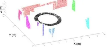
In the same room, the panoramic Leica HDS6100 laser scanner was used to capture four 360o scans from two different locations. All scans were levelled via the built-in electronic tilt sensor and have a different heading of 0o, 90o, 180o, and 270o. For the plane-based self-calibration a total of 69 planes were manually selected from the point cloud, each having a different position and orientation (Figure 15). The dimensions of the planes normally do not exceed two metres.
Figure 15: Sample of planar features extracted from the HDS6100 point cloud for use in the plane-based calibration.
Table 6 shows the systematic error terms found to be statistically significant from the plane-based self-calibration, using either 50 points or a maximum of 5000 points on each plane. The results from a point-based self-calibration using the same data are also included. The sensor only showed minor signs of laser axis vertical offset (a2) and non-orthogonality of horizontal encoder circle and vertical axis (b4 and b5). The results demonstrate that the plane-based calibration can recover the same systematic errors as the point-based self-calibration
but with even greater precision, mainly due to the higher degrees of freedom (d.o.f.). For computational efficiency in the calibration, the results from using only 50 points on each plane can be used as it will not be significantly different from using a maximum of 5000 points on each plane.
Table 6: Systematic error terms for the HDS6100 calibration Plane (5000 pts) Plane (50 pts) Targets (104)
d.o.f. 724569 10616 531
value σ value σ value σ
a2 [mm] -1.05 0.02 -1.09 0.12 -1.38 0.59
b4[“] 6.28 0.21 6.76 1.50 7.97 4.02
b5[“] 7.12 0.21 10.19 1.46 13.41 3.72
5. CONCLUSION
The TLS calibration model and knowledge developed in point-based calibration is transferable to plane-point-based self-calibration. All of the four most prominent errors in TLS instruments behave more or less in the same manner in both point-based and plane-based calibration for both panoramic and hybrid type laser scanners. Some new correlations were discovered (e.g. collimation axis error in hybrid scanners) that act differently in the plane-based calibration, but some mitigation developed from the point-based calibration is still applicable. The recovery of the collimation axis error for hybrid scanners has always posed a challenge in previous studies and will remain a topic for future investigation in plane-based self-calibration. The real data captured with the GS200 showed that the raw measurement precision of the system can be improved through the plane-based calibration. The calibration of the HDS6100 reinforced the concept that both point-based and plane-based self-calibrations can achieve similar results. The systematic errors recovered using either method are not significantly different and show that the plane-based calibration can be carried out with a low density point cloud.
ACKNOWLEDGEMENTS
The authors would like to thank Natural Sciences and Engineering Research Council of Canada (NSERC) and Alberta Innovates for funding and supporting this research project. Thanks to Kathleen Ang and Claudius Schmit for their generous help with acquiring the HDS6100 data, and Kathleen for proof-reading this paper.
REFERENCES
Amiri Parian, J., & Grün, A. (2005). Integrated laser scanner and intensity image calibration and accuracy assessment. The International Archives of the Photogrammetry, Remote Sensing and Spatial Information Sciences 36 (Part3/W19), 18-23.
Bae, K., & Lichti, D. (2007). On-site self-calibration using planar features for terrestrial laser scanners. The international Archives of the Photogrammery, Remote Sensing and Spatial Information Sciences 36 (Part 3/W52), 14-19.
Chow, J., Lichti, D., & Teskey, W. (2010a). Self-calibration of the Trimble (Mensi) GS200 terrestrial laser scanner. The International Archives of the Photogrammery, Remote Sensing and Spatial Information Sciences 38 (Part 5), 161-166.
Chow, J., Teskey, W., & Lichti, D. ( 2010b). Self-calibration and evaluation of the Trimble GX terrestrial laser scanner. The International Archives of the Photogrammery, Remote Sensing and Spatial Information Sciences 38 (Part 1).
Dorninger, P., Nothegger, C., Pfeifer, N., & Molnár, G. (2008). On-the-job detection and correction of systematic cyclic distance measurement errors of terrestrial laser scanners. Journal of Applied Geodesy 2 (4), 191-204.
Förstner, W.; Wrobel, B. (2004). Mathematical concepts in photogrammetry. In Manual of Photogrammetry, 5th ed.; McGlone, J.C., Mikhail, E.M., Bethel, J., Mullen, R., Eds.; American Society of Photogrammetry and Remote Sensing: Bethesda, MD, USA, pp. 15-180.
Gielsdorf, F., Rietdorf, A., & Gruendig, L. (2004). A Concept forthe calibration of terrestrial laser scanners. In: Proceedings of the FIG Working Week. Athens, Greece. [On CD-ROM].
Glennie, C., & Lichti, D. (2010). Static calibration and analysis of the Velodyne HDL-64E S2 for high accuracy mobile scanning. Remote Sensing 2 (6), 1610-1624.
González-Aguilera, D., Rodríguez-Gonzálvez, P., Armesto, J., & Arias, P. (2011). Trimble GX200 and Riegl LMS-Z390i sensor self-calibration. Optics Express 19(3), 2676-2693.
Lichti, D. (2007). Modelling, calibration and analysis of an AM-CW terrestrial laser scanner. ISPRS Journal of Photogrammetry and Remote Sensing 61 (5), 307-324.
Lichti, D. (2010). Terrestrial laser scanner self-calibration: correlation sources and their mitigation. ISPRS Journal of Photogrammetry and Remote Sensing 65 (1) , 93-102.
Lichti, D., Chow, J., & Lahamy, H. (2011). Parameter de-correlation and model-identification in hybrid-style terrestrial laser scanner self-calibration . ISPRS Journal of Photogrammetry and Remote Sensing, 66 (3), 317-326.
Molnár, G., Pfeifer, N., Ressl, C., Dorninger, P., & Nothegger, C. (2009). Range calibration of terrestrial laser scanners with piecewise linear functions. Photogrammetrie, Fernerkundung, Geoinformation 1, 9-21.
Reshetyuk, Y. (2006). Calibration of terrestrial laser scanners callidus 1.1, Leica HDS 3000 and Leica HDS 2500. Survey Review 38 (302).
Reshetyuk, Y. (2009). Self-calibration and direct georeferencing in terrestrial laser scanning. Doctoral Thesis. Department of Transport and Economics, Division of Geodesy, Royal Institute of Technology (KTH), Stockholm, Sweden, January.
Reshetyuk, Y. (2010). A unified approach to self-calibration of terrestrial laser scanners. ISPRS Journal of Photogrammetry and Remote Sensing 65 (5), 445-456.
Rieger, P., Studnicka, N., Pfennigbauer, M., & Zach, G. (2010). Boresight alignment method for mobile laser scanning systems. Journal of Applied Geodesy 4 (1), 13-21.
Schneider, D., & Schwalbe, E. (2008). Integrated processing of terrestrial laser scanner data and fisheye-camera image data. The International Archives of the Photogrammetry, Remote Sensing and Spatial Information Sciences 37 (Part B5), 1037-1043.
Skaloud, J., & Lichti, D. (2006). Rigorous approach to bore-sight self-calibration in airborne laser scanning. ISPRS Journal of Photogrammetry and Remote Sensing 61 (1), 47-59.
Soudarissanane, S., Lindenbergh, R., Menenti, M., & Teunissen, P. (2011). Scanning geometry: Influencing factor on the quality of terrestrial laser scanning points. ISPRS Journal of Photogrammetry and Remote Sensing, DOI: 10.1016/j.isprsjprs.2011.01.005. (In Press).