Journal of Economic Dynamics & Control 25 (2001) 1}34
The CO
2
abatement game: Costs, incentives,
and the enforceability of a sub-global
coalition
qMustafa H. Babiker
Joint Program on the Science and Policy of Global Change, MIT-E40-267, Cambridge, MA 02139, USA
Abstract
This paper studies the economic incentives and the institutional issues governing the
outcomes of a short-term climate change policy package guided by the United Nations'
Framework Convention on Climate Change and the Berlin Mandate initiatives. Game theoretic tools and the global trade-environment interface are explored within a 26-region, 13-commodity computable general equilibrium framework to characterize the incentives of OECD regions to comply with a non-binding agreement in a carbon abatement coalition. The results showed that, in the absence of side payments, the achievement of such a coalition might require the design of suitable trade
instru-ments. ( 2001 Elsevier Science B.V. All rights reserved.
1. Introduction
Increased concern about the possibility of an irreversible global climate change has resulted in several international initiatives that may ultimately lead to adoption of policies to reduce greenhouse gas emissions. The signing of the United Nations' Framework Convention on Climate Change (FCCC), the Berlin Mandate, and the Kyoto Accord are major steps in this direction. In its
q
I thank Thomas Rutherford, Yongmin Chen, Mark Cronshaw, Nicholas Flores, John Reilly, and two anonymous referees for helpful comments.
E-mail address:[email protected] (M.H. Babiker).
1Annex1 consists of OECD countries, Former Soviet Union and the East European countries. In this paper our focus is on OECD only.
2Examples of the game theoretic literature are Maler (1991), Barrett (1991,1994), Carraro and Siniscalo (1993), Heal (1994), and Sandler and Sargent (1995).
3For example the global warming game in Maler (1991) is a Prisoner's dilemma, in Carraro and Siniscalo (1993) is a supergame with possibly stable partial coalitions, and in Sandler and Sargent (1995) is a coordination game in which both mutual defection and full cooperation are Nash equilibria. Characterizing it slightly di!erent, Heal (1994) motivates the formation of critical coalitions and establishes the su$cient conditions for their stability; yet these conditions implicitly preclude the presence of strong free rider incentives among the coalition members.
4Most of the empirical literature on global warming has emerged from numerical general equilibrium models, e.g. Whalley and Wigle (1991), Manne and Richel (1992), Perroni and Ruthe-rford (1993), Piggott et al. (1993), Larsen and Shah (1994), OECD (1995), and Harrison and Rutherford (1997).
fourth article, the FCCC calls upon Annex11countries to take early actions to stabilize their greenhouse gas (GHG) emissions to their 1990 levels by year 2000. The Berlin Mandate has included a number of proposals each suggesting 10}20% reductions in Annex1's GHG emissions from their 1990 levels by year 2010. Whereas the recent agreement in Kyoto requires the European Union to reduce them by 8%, the US by 7%, and Japan by 6% during the period 2008}2012. Nevertheless, it remains unclear whether and how the policy recom-mendations of these initiatives may be implemented. Of central importance are two issues:"rst, will Annex1 voluntarily comply with some non-binding agree-ment in a coalition to reduce GHG emissions? And second, what institutional arrangements can be made that would promote cooperation among countries to achieve the emissions-reduction objective?
in which the welfare costs of abatement are equated across the members. Nevertheless, neither the maximum consensus cutbacks nor the burden sharing arrangements, by themselves, are su$cient to ensure the self-enforceability needed to stabilize the arrangement outcomes. In particular, the maximum consensus cutback in Piggott et al is based on bene"ciality, i.e. the cutback should be bene"cial to the coalition members, which is a necessary but not su$cient condition for the stability of the coalition.
This paper uses a game-theoretic framework and a computable general equilibrium (CGE) model to empirically quantify and assess the incentives of Annex1 countries to voluntarily comply with a non-binding agreement to form a CO
2-abatement coalition. The multi-region, multi-commodity CGE model is
developed to numerically simulate the strategic interactions among member countries in the di!erent coalition structures and to compute payo!s. I show that free riding incentives are so pervasive that a self-enforcing coalition is not supportable as an equilibrium outcome under the current institutional arrange-ments. I then consider linking climate and trade policy in a combined game to explore the implication of trade measures as enforcement mechanisms. I show that the Annex1 coalition can be supported as a subgame perfect equilibrium if suitable trade rewards and punishment instruments are designed.
The rest of the paper is organized as follows. Section 2, the analytical framework, describes our computable general equilibrium model (CGE) and the calibration of the carbon abatement bene"t functions. Section 3 provides a nu-merical assessment of welfare costs, institutions, and quota allocation rules in a 25%-cutback OECD coalition. Section 4 analyses the equilibria of the one-shot abatement game. Section 5 presents the repeated CO
2-game analysis and
explores the trade interaction as an enforcement mechanism. Section 6 provides concluding remarks.
2. The analytical framework
2.1. General setup
Consider a group of N countries contemplating an agreement to provide a speci"ed level of a pure public good (CO
2-abatement) through multi-lateral
negotiations. Let =
r be the welfare index for the rth country. Since the
abatement is a pure public good we assume=
r to have the special form: =
r";r(Cr(>r,pr,q))#Br(A), (1)
where;
ris the indirect utility index de"ned over income and prices throughCr,
C
ris a private consumption vector,Br is regionr's abatement bene"t function,
andAis the global CO
2abatement given by the summation technology:
A"+
s
a
s, (2)
5In the empirical construct only a subset of the N countries is contemplating to form the abatement coalition. In that case for the non-colluding countries abatement is unrestricted and their bene"ts from abatement are assumed to be zeros.
wheresdenotes regions and thea
s's are net regional CO2-abatements over the
no-agreement case (i.e. alla
s's are zeros in the status quo).pr is the domestic
price vector,qis the international price vector, and>
ris the net output vector
(GNP) de"ned by the transformation
>
r">(pr,q;ar). (3)
The functions;
r,Cr,Br, and>r are assumed to be well-behaved; in
particu-lar,>
r is non increasing inar, andBr is non decreasing inA.
Provided that=
r is separable in;r andBr, the regional abatement bene"t
functions may be evaluated independently of the private good technology. This is useful because the welfare cost (i.e. the loss in private consumption) of any abatement policy can be assessed with reasonable certainty given the observed regional production, consumption, and bilateral trade#ows. In contrast, due to the uncertainties surrounding the bene"ts side (see Cline, 1992; Nordhaus, 1993), it is extremely di$cult to model the bene"ts from reducing global warming within the household choice set. Having made these simplifying assumptions, we may proceed to solve the household optimization problem and measure the welfare costs implied by the given abatement policy. Next, we may use any reasonable exogenous estimates of the regional valuations to compute their total bene"ts from the resulting global abatement e!ort. The net regional gains from the given abatement policy would then be obtained by combining their corresponding cost and bene"t estimates.
Formally, leta6r be the abatement quota of regionrunder the agreement5. Complying with the agreement, the representative agent in each country, r, solves
max
cr ;
r(Cr(>r,pr,q)) (4)
s.t.
>
r">(pr,q;ar) ar5a6r.
In a multi-regional equilibrium framework, the solution to such a problem is characterized by the regional equilibrium price vectorpH
r, the regional
equilib-rium allocationsCH
r and>Hr, the regional shadow price vector associated with
the CO
2constraint, and the equilibrium international price vectorqH, such that
6The primary source for base year (1992) economic statistics is Global Trade Analysis Program (GTAP; see McDougall, 1997), and our primary source for energy demand, supply and price data is the OECD/IEA publications for 1992.
equilibrium problem is formulated and solved as a CGE model using the GAMS/MPSGE software described in Rutherford (1995,1999).
2.2. An overview of the CGE model and its implementation
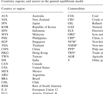
The framework is a static multi-regional general equilibrium model of energy and trade. The model is built on a comprehensive energy-economy dataset that accommodates a consistent representation of energy markets in physical units as well as detailed accounts of regional production and bilateral trade #ows (Rutherford and Babiker, 1997). The analysis covers 26 regions and 13 sectors, the description of which is provided in Table 1.
The sectoral aggregation scheme was chosen to return carbon-intensive industries as separate sectors.6The energy goods identi"ed in the model include coal (COL), gas (GAS), crude oil (CRU), re"ned oil products (OIL) and electric-ity (ELE). This disaggregation is essential in order to distinguish energy goods by carbon intensity and by the degree of substitutability. In addition, the model features important carbon-intensive and energy-intensive industries which are potentially those most a!ected by carbon abatement policies, such as Iron and steel (ORE), chemical products (CRP), non-ferrous metals (NFM), non-metallic minerals (NMM), pulp and paper (PPP), and trade and transportation services (TRN). The rest of the economy is divided into agricultural production (AGR) and other goods (Y).
Primary factors include labor, capital, land and fossil}fuel resources. Labor and capital are treated as perfectly mobile across sectors within each region but internationally immobile. The production functions assumed in each sector allow su$cient levels of nesting to permit substitution between primary energy types, as well as substitution between a primary energy composite and second-ary energy (electricity).
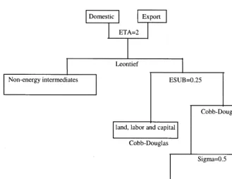
Fig. 1 illustrates the nesting structure employed for production sectors other than fossil fuels. Output is produced with"xed-coe$cient (Leontief) inputs of intermediate non-energy goods, and an energy-primary factor composite. The energy composite is in turn produced with a constant-elasticity-of-substitution (CES) function of a energy composite and electricity. The primary-energy composite is then a function of coal, crude oil, re"ned oil and natural gas. The value-added composite consists of a Cobb}Douglas aggregation of labor, capital and land.
Table 1
Countries, regions, and sectors in the general equilibrium model
Country or region Commodities
AUS Australia COL Coal
NZL New Zealand CRU Crude oil
JPN Japan OIL Re"ned oil products
KOR Republic of Korea GAS Natural gas
IDN Indonesia ELE Electricity
MYS Malaysia ORE! Iron and steel
PHL Philippines CRP! Chem, rubber and plastic
SGP Singapore NFM! Non-ferrous metals
THA Thailand NMM! Non-metallic minerals
CHN China PPP! Pulp and paper
HKG Hong Kong TRN! Trade and transport
TWN Taiwan AGR Agricultural goods
IDI India Y Other goods
CAN Canada
USA United States
MEX Mexico
ARG Argentina
BRA Brazil
CHL Chile
RSM Rest of South America E}U European Union 12 EU3 Austria, Finland, &
Sweden
FSU Former Soviet Union
MEA Middle East & North Africa
SSA Sub-Saharan Africa
ROW Rest of World
!Energy-intensive goods.
7The energy demand elasticities used in the model are consistent with those typically used in the literature, and are within the ranges reported in econometric studies (e.g. Pindyck, 1979; Nguyen, 1986; Nainar, 1989).
model, where the substitution elasticity between the speci"c factor and the composite is calibrated to match an exogenous fossil fuel supply elasticity. The supply elasticities used in the model are 2 for crude oil, 0.5 for coal, and 1 for natural gas.
Fig. 1. Structure of non-fossil fuel production.
Fig. 2. Nesting structure for"nal demand.
CO
2emissions are associated with fossil fuel consumption in production and
"nal demand. Di!erent fuels have di!erent carbon intensities. The technology producing CO
2, then, is a"xed proportion activity in which each unit of a fuel
abatement, other than reducing consumption, are inter-fuel and fuel-non fuel substitutions.
The model's equilibrium framework is based on"nal demands for goods and services in each region arising from a representative agent. Final demands are subject to an income balance constraint with"xed investment. Consumption within each region is "nanced from factor income, taxes and exogenously speci"ed capital #ows. Taxes apply to energy demand, factor income and international trade, and these "nance a "xed level of public provision. The government budget is balanced through lump-sum taxes.
Energy goods and other commodities are traded in world markets. Crude oil is imported and exported as a homogeneous product, subject to tari!s and export taxes. All other goods, including energy products such as coal, electricity, and natural gas, are characterized by product di!erentiation with an explicit representation of bilateral trade#ows calibrated to trade#ows for the reference year, 1992.
Energy products (re"ned oil, coal, natural gas, and electricity) are sold at di!erent prices to industrial customers and "nal consumers. The physical quantities of sectoral and"nal energy demand are calibrated to the OECD/IEA Energy Balances and Statistics. The essential features of the model formulation are provided in Appendix A and the full mixed complemenarity formulation (MCP) in Appendix B.
2.3. The calibration of CO2-abatement benext functions
Following Hoel (1991), Nordhaus (1993), and Barrett (1994), two functional forms ofB
r are speci"ed:
B
r(A)"brA, br50 (5)
B
r(A)"jrA!crA2, j'0, c'0 (6)
Where from (5) the marginal bene"t in countryris the constantbr, and from (6) the marginal bene"t is the downward sloped linear functionjr!2crA. Given the global abatement level A from the agreement and the solution of the household problem, the evaluation of the bene"ts from abatement reduces to the determination of the constantsb
r,jr, andcr.
8However, some preliminary sensitivity analyses have shown that the main insights of the paper are not a!ected by the size of the target.
damage from the doubling of CO
2 atmospheric concentration is about 1% of
1990 GDP, whereas Fankhauser (1993) suggests the world annual damage for the same scenario to be about 1.4% of the world 1990 GDP. On the mitigation cost side, the simulations of the GREEN model (OECD, 1995) suggest that the world average annual GDP loss from stabilizing CO
2emissions in Annex1 to
their 1990 level is about 1%.
Based on this, two estimates of the regional per-capita marginal bene"ts (or marginal willingness to pay) are considered in our numerical simulations. The "rst estimate assumes the per-capita marginal bene"t for each country is 5% higher than the country's corresponding per-capita welfare cost (in dollars) of mitigation. We call this estimate =0. The second estimate assumes identical
per-capita marginal valuations across all the parties, and calibrates the marginal bene"t coe$cient (br) to be 1% higher than the highest regional per-capita welfare cost of mitigation. On the other hand,jr andcr in the linear marginal bene"t formulation are calibrated using the estimates ofbr in such a way that the individual marginal willingness to pay declines by$100 for each additional billion tons of CO
2abated. We call the linearized version of the second estimate
=1.
3. A 25%-cutback OECD carbon coalition
3.1. Current policy climate and model scenarios
According to the 1992 projections of the Intergovernmental Panel on Climate Change (IPCC), fossil fuel CO
2-emissions are likely to grow by 2.5}3.5%
annually in the business-as-usual (BaU) trajectories. Since CO
2 is the major
anthropogenic greenhouse gas any short-term abatement action will naturally focus on it. Given the GHG reduction targets in Berlin and Kyoto along with the IPCC projections, we"nd 25% cutback from the 1992 CO
2-emissions level
in OECD to be a good approximation of these targets in a static setting.8Such an abatement e!ort, in turn, is equivalent to a global reduction of 12% according to the IEA 1992 statistics.
To simplify the computation of payo!s, the 7 OECD regions in the original dataset are aggregated into 5 regions: AUS Australia and New Zealand, JPN Japan, CAN Canada, USA United States, and E}U European Union as de"ned in 1990 plus EU3. The observed 1992 fossil fuel CO
2-emissions in OECD are
9Following the arguments in Schelling (1992) of the political implausibility of an international carbon tax, a uniform OECD carbon tax is not considered in the analysis.
10To check how close our 25% OECD cut approximates the e!ect of the FCCC and Berlin Mandate: for a grandfathering scenario in which the FCCC global target is wholly met by OECD through a uniform tax, the simulations of the OECD GREEN model suggest that the OECD average real income loss over the period 1990}2050 is 0.76% relative to the business as usual baseline. In contrast, the results on Table 2 (for the grandfathering with uniform permit) indicate an OECD loss of 0.57% of the 1992 GDP.
issues, both the FCCC and Berlin Mandate seem to have endorsed economic e$ciency, equity, gradual action, and wider coalition as appropriate climate policy responses. E$ciency, equity, and cost sharing issues among the OECD regions are addressed through institution and quota allocation rule scenarios. Two types of institutional arrangements are simulated: A uniform OECD permit market and regional permit markets.9 Four rules for allocating CO
2
emission rights are experimented: The"rst emphasizes the status quo (Grand-fathering) and the other three emphasize equity, carbon e$ciency, and per-capita cost sharing.
3.2. Institutions,quota rules,and welfare impacts in a unilateral OECD abatement coalition: Simulation results
Table 2 presents a summary of the simulation results on institutions and quota allocation rules. The grandfathering rule, columns (1) and (2), allocates members'quotas in proportion to their 1992 CO
2-emissions (this is equivalent
to each OECD region cutting its emissions by 25%); the egalitarian rule, column (3), allocates the members'quotas in proportion to their 1992 populations; the carbon e$ciency rule, column (4), allocates the members'quotas in proportion to their 1992 CO
2-intensities per unit of their corresponding per-capita GDPs;
and the cost sharing rule, column (5), assigns members'quotas in such a way that per-capita welfare costs (in dollars) are equated across the coalition mem-bers. The welfare costs are expressed in three forms: the percentage change in the Hicksian index, EV%, the per-capita consumption reduction in dollars, and the regional forgone consumption as a percent of the 1992 regional GDP.10Along with these, Table 2 also reports trade #ows in CO
2-permit market for the
di!erent allocation rules. In terms of institution design, the results in columns (1) and (2) suggest that the movement into a uniform permit market is a Pareto-improvement for every member (assuming away transaction costs.) This im-provement is a result of both the lower abatement cost and the lower leakage rate (the increase in CO
2-emissions by non-abating countries as a percentage of
Table 2
Quota allocation rules, institutions, and the welfare impacts of an OECD CO
2Coalition
(1)! (2)" (3)#
Grand fathering, no permit market Grandfathering, with permit market Egalitarian, with permit market
Welfare costs Welfare costs Welfare costs CO
2$
Region EV% $percap % gdp Quota % Ev% $percap % gdp CO
2$
Trade B$
Quota % EV% $percap % gdp
Trade B$
AUS 1.5 150 0.9 2.9 0.7 72 0.5 2.9 2.9 0.5 50 0.3 3.4
JPN 0.7 115 0.4 11.5 0.7 112 0.4 !3.5 17.3 !1.7 !278 !0.9 38.0
CAN 1.4 168 0.8 4.3 1.3 156 0.8 1.8 4.0 2.3 276 1.4 0.5
USA 1.1 161 0.7 48.0 0.9 142 0.6 15.1 35.6 3.6 554 2.4 !74.5
E}U 1.1 172 0.7 33.3 1.0 163 0.6 !16.3 40.2 !0.2 !29 !0.1 33.6
OECD 1.0 157 0.6 100 0.9 144 0.57 0 100 1.0 150 0.6 0
(4)% (5)&
Carbon-e$ciency with permit market Cost-sharing, with permit market
Welfare costs Welfare costs
Region Quota % EV % $percap % gdp CO
2$
Trade B$
Quota % EV % $percap % gdp CO
2$
Trade B$
AUS 1.7 5.3 527 3.3 !4.6 2.7 1.5 144 0.8 2.4
JPN 27.6 !5.6 !935 !3.2 108.2 11.1 0.9 144 0.5 !6.8
CAN 2.6 5.7 674 3.4 !10.3 4.4 1.2 144 0.7 2.3
USA 22.1 6.5 1000 4.3 !165.8 47.9 0.9 144 0.6 13.7
E}U 46.0 !1.2 !186 !0.7 72.5 33.9 0.9 144 0.5 !11.6
OECD 100 1.1 162 0.65 0 100 0.9 144 0.57 0
!Leakage 12.5%, net global CO
2abatement 10.4%.
"Leakage 11.5%, net global CO2abatement 10.6%. #Leakage 11.7%, net global CO2abatement 10.5%. $Indicates permit purchase.
%Leakage 11.8%, net global CO2abatement 10.5%. &Leakage 11.5%, net global CO2abatement 10.6%.
M.H.
Babiker
/
Journal
of
Economic
Dynamics
&
Control
25
(2001)
1
}
34
With respect to quota rules, both the equity and the e$ciency criteria result in higher emission quotas for JPN and E}U, and lower ones for AUS, CAN, and USA compared to those assigned by the grandfathering rule. This is because both JPN and E}U are relatively more energy e$cient and relatively more populated than their other OECD partners. The welfare impacts for these two rules are shown respectively in columns (3) and (4). It is clear from the statistics that JPN and E}U are net gainers, whereas AUS, CAN, and USA appear to experience huge welfare losses. Not only that, but the overall OECD welfare, measured by a base- year-consumption weighted Hicksian index, is lower and the leakage rate is higher for either of these two rules when compared to the corresponding results from the grandfathering rule. Based on these results, an OECD CO
2-coalition
with quotas allocated according to either a pure egalitarian criterion or a pure e$ciency criterion is unlikely. The last rule simulated in the analysis is the per-capita cost-sharing allocation. The simulation results for this allocation are displayed on column (5). The corresponding quotas implied by this rule suggest a minor reallocation of the grandfathering quotas from the relatively low welfare cost members (AUS,JPN, and USA) to the relatively high welfare cost ones (CAN and E}U). In terms of the overall performance (i.e. OECD welfare and leakage rate), the results for this allocation are identical to those of the grandfathering allocation i.e. the two allocations seem to lie on the same OECD Pareto-frontier. The main insights from the exercises in Table 2 are therefore: (i) a uniform permit market is better than having separate regional permit markets or tax arrangements; (ii) quota allocation rules that favor e$ciency or egalitarian criteria are unlikely; and (iii) irrespective of the institution type or the quota rule, there are likely to be sharp di!erences in the welfare impacts of the abatement policy across the OECD regions.
To provide insights on the curvature of the marginal abatement costs and to motivate the game analyses in the following sections, we have computed the uniform permit price and the regional per-capita welfare costs for several reduction targets in the range 0}40%. The implied elasticities suggest that the marginal abatement cost curves are quite steep. The CO
2-abatement elasticity
with respect to the coalition permit price is found to range between 0.04 and 0.13, and that with respect to the regional per-capita welfare costs is found to range between 0.01 and 0.15. The presence of such steep marginal abatement costs implies free riding incentives are likely to be huge and consequently the chances for a self-enforcing OECD abatement coalition are small.
4. The one-shot game analysis and the stability of an OECD carbon coalition
4.1. Benext estimates and payows
grandfathering with uniform permit scenario, =0 corresponds to a 5%
markup on the regional per-capita welfare costs shown for the scenario in Table 2, whereas=1 corresponds to the linearized version of a 1% markup
on the highest regional per-capita welfare cost shown for the scenario on the same table (namely that of E}U). The regional total bene"ts from the cutback implied by these estimates lie in the range 0.4}0.9% of the correspond-ing 1992 regional GDPs. To express the capita bene"t estimates in per-billion tons of CO
2 terms, we divide by the coalition net abatement (i.e.
abatement-leakage).
4.2. Equilibria in the one-shot OECD-coalition game
The one-shot OECD interaction is a complete-information simultaneous move game in which each region has two strategies: C cooperate (i.e. comply with the abatement agreement), and N not-cooperate (i.e. not comply with the agreement). All players (i.e. OECD regions) are rational (i.e. welfare maximizers), and for every player: both the other players'strategies and the game payo!s are known. The simulated payo!s for the game constructs with grandfather-ing#permit scenario are reported in Table 3, where players are labeled A for AUS, J for JPN, D for CAN, U for USA, and E for E}U, and where payo!s correspond to players on the column.
Note that the strategies for the row players are ordered in accordance with the ordering of the players, e.g., strategies NCNC and row players JDUE means J plays N, D plays C, U plays N, and E plays C.
Since by construction the values of=0 and=1 that correspond to the
full-cooperation entries are predetermined, one can infer nothing about the actual bene"t from full-cooperation on their basis. Nevertheless, relative to whatever benchmarking is used for the full-cooperation con"guration, the rest of the entries are valid payo!s for assessing the regional incentives for cooperation and defection.
For both the =0 and =1 games, except for AUS, the net bene"t from
not cooperating for each of the OECD regions, given that the other four regions cooperate, is greater than the corresponding net bene"t from co-operating. Hence, by the de"nition of Nash equilibrium, full-cooperation is certainly not an equilibrium in either of the two games, and accordingly none of these games is a coordination one. Next, by looking at the individual region payo!columns that correspond to its strategies C and N, we see in both
=0 and=1 games that the payo!s from N strictly exceed those from C for all
regions except AUS. But by the concept of iterative dominance, the relevant payo!s facing AUS in the two games would, respectively, then be!1.2,!1.1 for C, and 0,0 for N. Then the only equilibria for the=0 and the=1 games are
OECD-coalition game payo!s (b$) scenario: grandfathering#OECD permit market!
(a)The game based on=0benext estimate
Column player A J D U E
Row players JDUE ADUE AJUE AJDE AJDU
Strategy C N C N C N C N C N
CCCC 0.1 !0.0 0.7 20.2 0.2 2.8 1.8 13.5 2.3 35.4
NCCC 0.3 0.4 !0.2 19.2 0.1 2.6 1.0 11.9 0.1 34.2
CNCC 0.1 !0.1 !0.4 19.0 !0.2 2.4 !3.5 9.1 !4.9 28.6
CCNC 0.3 !0.9 !8.9 11.5 0.5 1.8 1.0 12.8 0.1 33.6
CCCN !0.2 0.3 !7.1 10.5 !1.4 1.3 !10.0 5.7 !25.5 10.4
NNCC 0.3 0.3 !1.4 18.0 !0.3 2.2 !4.3 7.6 !7.2 26.6
NCNC 0.6 !0.5 !9.8 10.7 0.7 1.5 0.3 10.6 !2.1 31.5
NCCN !0.0 0.7 !7.9 9.5 !1.4 1.1 !10.4 4.3 !27.7 8.4
CNNC 0.6 !1.0 !9.8 10.8 0.2 1.5 !4.4 8.4 !7.1 26.0
CNCN !0.2 0.3 !7.9 9.4 !1.6 1.0 !14.0 2.1 !32.2 3.7
CCNN !0.5 !0.4 !16.1 1.7 !1.6 0.4 !10.4 5.0 !26.7 8.8
NNNC 1.0 !0.5 !10.8 10.0 0.5 1.3 !5.1 6.8 !9.4 24.8
NNCN !0.1 0.6 !9.0 8.6 !1.7 0.9 !15.1 0.7 !34.6 1.7
NCNN !1.0 0.0 !17.8 0.8 !1.4 0.2 !11.4 3.7 !29.5 6.9
CNNN !0.1 !0.4 !17.5 0.9 !2.3 0.1 !15.1 1.3 !33.6 1.9
NNNN !1.2 0 !19.5 0 !2.4 0 !15.6 0 !35.5 0
(b)The game based on the=1benext estimate
CCCC 2.3 2.2 8.9 27.6 0.8 3.3 10.6 18.7 5.8 38.9
NCCC 2.3 2.3 7.8 26.4 0.7 3.1 9.7 16.8 3.6 37.6
CNCC 2.2 2.0 7.5 26.1 0.4 2.9 4.7 13.2 !1.3 31.9
CCNC 1.4 0.2 !4.6 14.8 0.9 2.1 9.6 17.7 3.7 37.0
CCCN 1.4 1.8 !1.2 15.6 !0.9 1.7 !3.2 7.8 !22.6 11.7
M.H.
Babiker
/
Journal
of
Economic
Dynamics
&
Control
25
(2001)
1
}
NNCC 2.2 2.1 6.4 24.9 0.3 2.7 3.7 11.3 !3.6 29.8
NCNC 1.5 0.3 !5.7 13.8 1.1 1.9 8.7 15.0 1.5 34.9
NCCN 1.3 1.9 !2.1 14.4 !1.0 1.5 !3.7 6.0 !24.9 9.5
CNNC 1.6 !0.1 !5.7 13.8 0.5 1.8 3.5 12.1 !3.5 29.1
CNCN 1.3 1.7 !2.3 14.1 !1.2 1.4 !7.9 2.9 !29.8 4.2
CCNN !0.0 !0.0 !14.5 2.4 !1.5 0.5 !3.8 6.7 !23.9 9.8
NNNC 1.8 0.2 !7.2 12.8 0.8 1.6 2.6 10.2 !5.8 27.9
NNCN 1.2 1.8 !3.6 13.2 !1.3 1.3 !9.3 1.2 !32.4 2.0
NCNN !0.8 0.1 !16.5 1.2 !1.3 0.3 !5.0 5.0 !26.9 7.7
CNNN 0.2 !0.2 !16.2 1.2 !2.2 0.2 !9.5 1.7 !31.3 2.2
NNNN !1.0 0 !18.5 0 !2.3 0 !10.1 0 !33.5 0
!Key:
Players: A AUS, J JPN, D CAN, U USA, and E E}U.
Strategies: C cooperate, N not cooperate; payo!s correspond to column players.
M.H.
Babiker
/
Journal
of
Economic
Dynamics
&
Control
25
(2001)
1
}
34
11This outcome is found to be largely insensitive to both the type of institution and the quota allocation rule. In particular we have simulated the=0 and the=1 games for the case of regional
permit markets and the case of per-capita cost sharing quota allocation rule and found that the mutual defection outcomes is the unique equilibrium in both cases.
12In the Piggott et al. language, these are the smallest coalitions for which the 25%-cut is aconsensus emission reduction.
the games corresponding to =0 and =1 belong to the Prisoner's dilemma
class.11
With respect to the feasibility of a stable (or a self-enforcing) sub-coalition, the preceding analysis suggests the prompt answer that the maximum size of such a sub-coalition is zero for both the=0 and=1 games. Alternatively, one may
ask the weaker version: Whether smaller bene"cial sub-coalitions are feasible, and what is the size of the smallest such sub-coalition?12By verifying that the sub-coalition must be bene"cial for every member, the smallest size that support such a principle is 5 for the =0-game (i.e. the minimum bene"cial size is full
cooperation) and 3 for the =1-game (namely JPN, USA, and E}U). This
suggests that a bene"cial OECD sub-coalition must include at least JPN, USA, and E}U.
A"nal piece of inference on the payo!s in Table 3 is the observation that defection incentives among the big OECD members (i.e. JPN, USA, and E}U) appear to be pairwise uncorrelated. This is important for the later repeated game analysis, because it precludes the possibility of e!ective coalitions among defectors.
Recognizing that these numerical outcomes are surrounded by uncertainties about the true elasticities governing the solution of the CGE model as well as uncertainties about the magnitudes of bene"t from slowing down global warm-ing, it is essential to carry out some sensitivity analysis to test the robustness of these outcomes. The critical elasticities in the CGE model include the crude oil supply elasticity, energy demand elasticities, and the Armington trade elastici-ties. We have simulated the=0 game for the low and high values of each of
Table 4
Sensitivity of free rider incentive to model elasticities (gains from unilateral defection b$)!
Oil supply Armington Energy demand
Low High Low High Low High
AUS !0.1 !0.1 !0.4 !0.3 !0.8 0.2
JPN 21.5 19.2 17.8 20.8 26.7 14.3
CAN 3.0 2.4 1.3 2.9 3.8 1.7
USA 13.8 11.3 8.7 12.1 24.3 5.7
E}U 36.5 32.8 32.9 33.8 54.1 20.0
!Scenario:=0 Game with Grandfathering#permit.
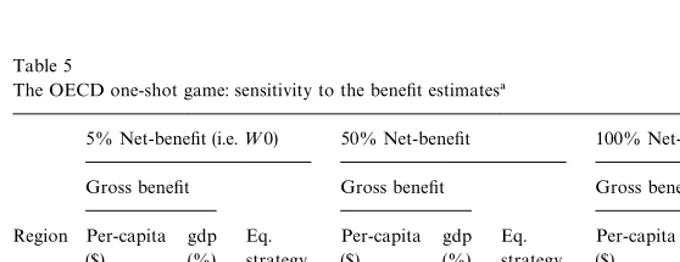
Table 5
The OECD one-shot game: sensitivity to the bene"t estimates!
5% Net-bene"t (i.e.=0) 50% Net-bene"t 100% Net-bene"t
Gross bene"t Gross bene"t Gross bene"t
Region Per-capita ($)
gdp (%)
Eq. strategy
Per-capita ($)
gdp (%)
Eq. strategy
Per-capita ($)
gdp (%)
Eq. strategy
AUS 75.6 0.53 N 108.0 0.75 N 144.0 1.0 N JPN 117.6 0.42 N 168.0 0.60 N 244.0 0.8 N CAN 163.8 0.84 N 234.0 1.20 N 302.0 1.6 N USA 149.1 0.63 N 213.0 0.90 N 284.0 1.2 C E}U 171.2 0.63 N 244.5 0.90 N 326.0 1.2 N
!Key:
Strategy: C Cooperate, N Not-cooperate; Scenario: Grandfathering#permit.
self-explanatory and clearly underscore the robustness of the mutual defection outcomes in the one-shot OECD coalition game.
To sum up, the likely equilibrium of the OECD one-shot coalition game seems to be the unavoidable Prisoner's dilemma mutual defections outcome. Under the current institutional arrangements and in the absence of a regional sovereign institution that enforces commitments, a stable and bene"cial carbon coalition among OECD regions is, therefore, unlikely. In the next section we motivate and present a repeated trade-environment framework, within which we show that a stable OECD coalition may be achieved.
13The two-phase construct is meant to capture the likeliness that, within the current climate policy regime, any agreement to be reached will be renegotiated after a decade or two.
14The regional discount factordris computed from the subgame-perfection condition: 1
1!d r
[Full-cooperation payo!]5[unilateral-defection payo!]
# dr
1!d r
[mutual-defection payo!].
5. Repeated game analysis:Trade-environment interface and subgame-perfection of the OECD CO2-coalition
In this section I"rst present the in"nitely repeated OECD coalition game and show that full-cooperation in such context is unlikely to be a subgame-perfect equilibrium outcome. Next, I motivate the connected trade-environment frame-work and present two constructs: The"rst is an in"nitely repeated trade-CO
2
interconnected game and the second is a two-phase super-game.13In the"rst construct, I show that cooperation in the full OECD coalition can be an equilibrium outcome if trade is included in the game. In the second, I character-ize a trade regime to support cooperation in the full OECD coalition during the "rst phase for relatively impatient players.
Note that for the remaining analysis in the paper, the focus shall be con"ned to the=0 with grandfathering#permit case.
5.1. The inxnitely repeated OECD CO2-game
Suppose the=0-game in Table 3 is to be repeated in"nitely with outcomes
from the previoust!1 periods,MtN=0, being observed before the start of periodt. Consider, for each OECD region, the following trigger strategy:
Play C in thexrst period. In period t, play C if every OECD region has played C in each of the t!1 previous periods; otherwise, play N.
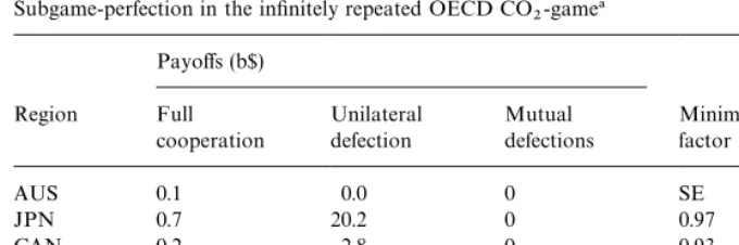
The regional minimum discount factors for which this trigger strategy consti-tutes a subgame-perfect Nash equilibrium of the in"nitely repeated game, together with the regional payo!s from full cooperation, unilateral defection, and mutual defections are reported in Table 6.14
Table 6
Subgame-perfection in the in"nitely repeated OECD CO
2-game!
Payo!s (b$) Region Full
cooperation
Unilateral defection
Mutual defections
Minimum discount factor [d
r]
AUS 0.1 0.0 0 SE
JPN 0.7 20.2 0 0.97
CAN 0.2 2.8 0 0.93
USA 1.8 13.5 0 0.87
E}U 2.3 35.4 0 0.94
!Key:
SE: cooperation is self-enforcing (best response). Scenario:=0 with grandfathering#permit.
15A detailed exposition on global warming*trade interface and the scope for an environment-based countervailing trade measures is provided in Whalley (1991) and Babiker et al. (1997).
16The recent Uruguay reforms are primarily meant to address this issue; nonetheless, they do not exhaust the room for further bene"cial trade coordination.
5.2. The repeated trade-environment connected framework
5.2.1. Motivation
The presence of global trade interaction and the subtleties of the global trade-environment interface15avail the players additional incentives to coordi-nate their actions as well as instruments to commit themselves to cooperation. The sub-optimality of the present global trading system,16the additional distor-tions injected by the presence of CO
2 taxes, and their associated repercussions
on competitiveness of energy-based industries and international trade #ows reinforce the need for further coordination of trade policies among the colluding parties. On the other hand, to set a&level playing"eld', players may be willing to take countervailing trade measures against defectors to limit the scope for environment trade-leakage and to punish free riding.
Motivated by the need of OECD regions to jointly coordinate their environ-mental actions with their trade policies, we think of a trade-CO
2interconnected
setup in which OECD regions negotiate a 25% reduction of tari!s on energy intensive imports along with the 25% CO
2-cutback. Within this setup, by
pooling the players'environment and trade incentives in one game, outcomes better than those in the isolated environment game may be achievable (Be-rnheim and Whinston, 1990).
Alternatively, we may think of a double-instruments trade strategy being added to the original CO
2-game in such a way that during the punishment
regime cooperation is rewarded by reduction of trade barriers and defection is punished by countervailing trade measures. Within such a context, our objective would be to characterize the extent of rewards and punishments needed to subgame-perfect the coalition. We consider these two constructs in turn:
5.2.2. The inxnitely repeated OECD trade-CO2 interconnected game
Suppose OECD regions agree to play the=0-game in Table 3, in which each
region has the strategiesMC,NN, jointly with a simultaneous move trade game, in which each OECD region has the strategies M¸,HN. ¸ says lower tari!s on
energy intensive imports by 25% and H says not lower them. The one-shot trade-CO
2 inter-connected game is then a simultaneous move game in which
each OECD region has the strategiesMC¸,CH,N¸,NHN, where in the status quoNHis being played by all regions.
Now, suppose this static interconnected game is to be repeated in"nitely with outcomes from all previous t!1 periods observed before the beginning of periodt. Next, for each OECD region, consider the trigger strategy:
Play CL in thexrst period. In period t, play CL if every OECD region has played CL in each of the t-1 previous periods; otherwise, play NH.
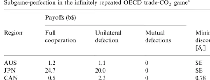
The regional minimum discount factors for which this trigger strategy constitutes a subgame-perfect Nash equilibrium of the in"nitely repeated trade-CO
2 game together with the regional payo!s from full-cooperation,
unilateral defection, and mutual defection are reported in Table 7. Where full cooperation means every region playing C¸, mutual defection means every region playing NH, and where the payo!s for unilateral defection are the maximum payo!s from unilaterally defecting in either or both the trade and the environment.
It is obvious that the minimum regional discount factors in Table 7 are on average 20% lower than those in Table 6. In particular, with the presence of trade coordination, Table 7 shows that environmental compliance is a best response for both AUS and JPN. Hence, this suggests that stronger subgame-perfection of the OECD carbon abatement coalition is achievable if trade coordination is invoked within the game than if not.
5.2.3. The two-phase OECD trade-CO2 connected super-game
Suppose the OECD regions agree to condition the play of the original
=0-game on a simultaneous move trade game, in which each region has the
Table 7
Subgame-perfection in the in"nitely repeated OECD trade-CO
2game!
Payo!s (b$) Region Full
cooperation
Unilateral defection
Mutual defections
Minimum discount factor [d
r]
AUS 1.2 1.1 0 SE
JPN 24.7 20.0 0 SE
CAN 0.5 2.3 0 0.78
USA 6.0 17.4 0 0.66
E}U 7.9 35.3 0 0.78
!Key:
SE: cooperation is self-enforcing (best response). Scenario:=0 with grandfathering#permit.
tari!on the CO
2content of the defecting region exports to the given region in
the coalition.
De"ne the two-phase repeated trade-CO
2 super-game construct as one in
which, within each phase, the=0-game and the trade game are played
simulta-neously each stage with the outcomes of the previous stage being observed before the beginning of the current stage. Let¹be the number of stages in the
"rst phase of the repeated super-game, and consider phase 2 to be in"nite. Within this construct, our interest is to characterize a subgame-perfect outcome in which cooperation on the CO
2-abatement is played by every OECD region
in each stage of the"rst phase, with the second phase providing the continuation of the punishment and reward regime.
Consider each OECD region adopting the following&3-instruments'strategy:
Play C and S in thexrst stage of phase 1. From the second stage on, play C and S if every region has played C and S in all the previous stages; otherwise, in addition to playing C, play R with those who have played C and S in all previous stages and play P with those who haven't. Punishment and rewards are carried over to phase 2.
Notice the two special properties of this strategy: (i) the trade instruments
RandP are to be played only when environmental defection is observed, i.e. they are essentially enforcement mechanisms. (ii) The mutual environmental defection is not invoked during the punishment regime, i.e., it avoids the implausible threat that every one defects.
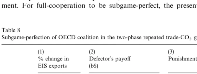
Table 8
Subgame-perfection of OECD coalition in the two-phase repeated trade-CO
2game!
(1) (2) (3)
% change in EIS exports
Defector's payo!
(b$)
Punishment regime
Def region Def Pun Def Cop Pun btax tari!red (%) Yr
AUS 75 !70 0.0 0.1 !0.9 1 10 1
JPN 7 !66 20.2 0.7 !2.9 2 50 11
CAN 33 !31 2.8 0.2 !7.8 1 25 2
USA 34 !65 13.5 1.8 !15.9 1 75 2
E}U 12 !99 35.4 2.3 !2.1 6 90 20
!Key:
EIS Energy intensive goods. Def Unilateral defection regime. Cop Cooperation regime.
Pun Cooperating and punishing the defector regime. btax Border CO
2 tax as a multiple of the coalition permit price.
tari!red % removal of tari!on EIS imports among colluding members. yr the required length of the region horizon.
Scenario: Grandfathering#permit, bene"t method=0.
instruments associated withRandP, and the horizon length such that playing the preceding strategy by every region constitutes a subgame-perfect Nash equilibrium of the"rst phase of the repeated super-game.
The countervailing tari!used in the numerical simulations is an endogenous tax on the CO
2-content of the defecting region exports to the remaining regions
in the coalition. In turn, the carbon content is measured by the per-dollar CO
2
coe$cients from the inverse input-output carbon computation, the details of which are described in Rutherford and Babiker (1997). We use a 10% discount rate for computing the regional horizon length. The simulation results for this exercise are summarized in Table 8.
Column (1) displays the percentage change in the defecting region's energy intensive exports (relative to their full-cooperation level) to the colluding re-gions. These are essentially the trade-leakage gains from free riding. As is apparent from &Def' entry, in the absence of punishment, these gains are considerable. In contrast, with the countervailing carbon tari!, these free rider gains are turned into losses (entry&Pun'). Nevertheless, for a large region such as E}U, the credibility of the punishment may call for a complete ban on its EIS exports to the coalition regions.
17Babiker (1998) shows that these requirements are substantially reduced if the coalition is expanded to include some of the non-OECD regions.
18Note that if we were to disaggregate the E}U region, these requirements could be quite reduced. Yet it is more plausible that the European countries will jointly coordinate their actions, and therefore it is more defensible to treat them as one player in the carbon abatement game. payo!s from cooperation for each member must be at least as high as that from unilateral defection followed by the punishment. For a 10% discount rate, entry &yr' of column (3) shows the region's minimum horizon needed to satisfy subgame-perfection of full-cooperation. As evident from the table, these hor-izons range from as low as 1 year for AUS to as high as 20 yr for E}U, suggesting that, given the punishment terms, a typical OECD decision maker, with a 20-yr planning horizon and who uses a 10% discount rate, would have no incentive to free ride. The&btax'entry in column (3) reports the per-ton border carbon tax expressed as a multiple of the corresponding coalition permit price. With exception to JPN and E}U, the results imply that an equal-foot treatment on trans-boundary carbon is a su$cient deterrent to free riding. The needed tari! reductions among the remaining parties in the coalition such that continuing cooperation and punishing the defector are best responses for each one, are in turn shown under entry &tari! red(%)' on column (3). The reported "gures suggest that tari!reductions in the range 10}90% could be called for if defection were to occur.17
Summing up, the results in Table 7 suggest that full cooperation among OECD regions can be fostered for relatively impatient policy makers if suitable trade reward and punishment instruments are designed, yet, the required reward and punishment patterns may prove to be quite stringent as they might amount to a complete ban on the imports from the defecting region.18
6. Concluding remarks
This paper has discussed some of the hot issues in the current global warming policy debate such as the design of institutions, the allocation of the abatement responsibilities, and the formation of CO
2-abatement coalitions. With respect
to the latter, the paper attempted to place the game theoretic analysis on global warming within an empirical context.
an abatement coalition to abate carbon emissions. Our analysis has shown that the unique outcome of the one-shot OECD abatement game is the status quo of no action. This outcome is shown to be quite robust with respect to both the damage and the mitigation cost parameters. In the absence of side payments and given the di$culty of commitment, some compliance mechanism is needed. Our results showed that full-cooperation among OECD regions can be supported as subgame-perfect equilibrium outcome and without invoking the implausible threat of mutual defections provided that appropriate trade punishment and reward instruments are included in the game. Nevertheless, the punishment terms may prove to be quite stringent as they might call for a complete ban of some trade with the defecting region.
7. For further reading
Cline, 1993; Farrell and Maskin, 1989; Swanson, 1991.
Appendix A. The algebraic structure of the CGE model
The model includes two types of production functions: Those for fossil fuels (crude oil, coal, and natural gas), and those for other goods. An index, >
*3,
characterizes the level of production for good iin region r, which (except for crude oil) is allocated to export and domestic markets according to a constant elasticity of transformation function
>
ir"
C
hirA
D
ir
D
ir
B
g# (1!h
ir)
A
X
ir
X
ir
B
g
D
1@g. (A.1)
Production of goods requires inputs of non-energy goods, energy-goods (oil, coal, gas, and electricity), and primary factors (labor, capital, and land). At the top level, non-energy goods and a constant-elasticity composite of primary factors and energy enter in"xed proportions:
>
ir"min
C
minj
G
x
jir
x6jir
H
, (airEoirE#(1!air)<oirE)1@oED
(A.2)in which the exponent determines the elasticity of substitution between primary factors and energy, p
E"1/(1!oE). Within this function, composite
energy E
ir is in turn a nested constant-elasticity composite of electric and
non-electric energy inputs, and <
ir is a Cobb}Douglas composite of capital,
labor, and land. Each fossil fuel input in the non-electric energy aggregate, is in turn a Leontief composite of an energy component and an associated CO
2
The representative consumer in regionrallocates income across alternative goods to solve
max ;
r(c)"
A
d<i|EC(irhioc)#(1!d)<ibECir(hioc)B
1@oc
s.t. +ip
irCir"Mr!pGrGr!pIrIr
(A.3)
in whichEis the set of energy goods entering"nal demand (oil, coal, gas, and electricity). Each fossil fuel inEis in turn, a"xed proportion composite of an energy and a CO
2component.dis the share of the consumption composite,h@is
are the expenditure shares in the corresponding composites, andM
r is region
rfactor earnings and tax revenue. Final demands for goods and services exhaust income net of expenditures on public goods and"nal investment, both of which are held constant in model.
Final and intermediate demands are nested CES composites of domestic and imported varieties:
C
ir"Cir
A
aDA
cDir
cDir
B
oD
#(1!a
D)
C
+s~r
h
s
A
cMisr
cMisr
B
c
D
oD@cB
1@oD.(A.4)
Here, the speci"c choices over domestic and imported demands are made to minimize unit cost (gross of applicable taxes):
min pDircDir#+
s(pXis(1#tXisr)#/isrpT)(1#tMisr)cMisr
s.t. f(cDir,cMisr)"C
ir.
(A.5)
In this equation,tXand tMare export and import taxes, and pTis the cost of international transportation services.
Appendix B. The mixed complimentarity formulation(MCP)
Data dexnition and model parameters
(a)Sets
I,i,j commodity set (13 commodities)
N,n non-energy goods (8 commodities)
E,e energy goods (5 commodities)
R,r,s regions (26 regions)
F,f factor inputs (land, labor, capital)
(b)Benchmark commodity taxes and prices
ty
i,r output tax
ti
j,i,r intermediate input tax
tx
i,s,r export tax rate
tm
i,s,r import tari!rate
tg
i,r tax rate on government consumption
tc
i,r tax rate on private consumption
tOMr tax rate on crude oil imports
tOXr tax rate on crude oil exports
PA0
j,i,r reference price of intermediates ["1#tij,i,r]
PMX0
i,s,r reference price of imports ["(1#txi,s,r)(1#tmi,s,r)]
PM¹0
i,s,r Reference price of transport services ["1#tmi,s,r]
PG0
i,r Reference price of government demand ["1#tgi,r]
PC0
i,r Reference price of private demand ["1#tci,r]
(c)Benchmarkvalue shares
dDi,r domestic market share of output
dIj,i,r intermediate input share
dVN,r value-added share in non-energy production
dSRE,r fossil fuel resource share
dOMr merchandise share in crude oil imports
dGr non-energy share in government demand
dCr non-energy share in private demand
hVf,i,r factor demand share in non-energy production
hGi,r government consumption share
hCi,r private consumption share
hTi,r intermediate demand share in transport
c
f,E,r factor demand shares in energy production
c
j,E,r intermediate demand shares in energy production
ai,r domestic production share in Armington aggregation
bMi,s,r import shares across regions
b9i,s,r merchandise component of imports (d)Elasticities and other parameters
pt domestic-export transformation elasticity
pV value-added-energy substitution elasticity
p%,r elasticity of substitution in energy production
pD Armington substitution elasticity
pM substitution elasticity across imports origin
p
G government energy-non-energy substitution elasticity
p
C private energy-non-energy substitution elasticity
G0
r benchmark government provision
FS0
&,r benchmark factor supplies
RS0
e,r benchmark supply of energy resource
Invest
i,r benchmark investment
Bopdef
r benchmark balance of payment de"cit
CO
%,r carbon coe$cient (kg/$)
Carblim
Model declarations
Variables
C
r private consumption
G
r government consumption >
i,r aggregate production
M
i,r import aggregation
A
i,r Armington supply
Oilm,
r crude oil imports
Oilx,
r crude oil exports
>¹ international transport service
CARB
r regional carbon emissions (billion tons)
P>
i,r price index of aggregate production
PD
i,r price index of production for domestic market
PX
i,r price index of production for exports
PM
i,r price index of aggregate imports
PE<
i,r price index of value added*energy aggregate
PA
i,r price index of Armington supply
PF
f,r price index of factor inputs
PR
e,r rent from energy-speci"c resource
PC
r price index of aggregate private consumption
PG
r price index of aggregate public provision
P¹ price index of international transport services
Pcrude international price of crude oil
Pcarb carbon permit price
Income
r regional income
Equations
PRF}C(R) private consumption zero-pro"t
PRF}G(R) public provision zero-pro"t
PRF}>(I,R) Aggregate output zero-pro"t
PRF}M(I,R) import aggregation zero-pro"t
PRF}A(I,R) Armington aggregation zero-pro"t
PRF}>¹ transport zero-pro"t
PRF}OM(R) import of crude oil zero-pro"t
PRF}OX(R) export of crude oil zero-pro"t
DEF}P>(I,R) de"nition of aggregate production cost
DEF}PE<(I,R) de"nition of energy-nonenergy price index
MK¹}PC(I,R) private consumption income-expenditure balance
MK¹}PG(R) public provision
MK¹}PD(I,R) clearance of domestic market
MK¹}PX(I,R) clearance of exports market
MK¹}PM(I,R) clearance of imports market
MK¹}PA(I,R) clearance for Armington supply
MK¹}PF(F,R) clearance of factor market
MK¹}PR(E,R) clearance of energy resource market
MK¹}P¹ clearance of international transport market
MK¹}CR;DE clearance of international crude oil market
MK¹}PCRB constraint on carbon emissions
CARB}DEF(R) regional carbon emissions
INC}RA(R) de"nition of regional income
Model equations
Zero-proxt conditions and dexnitions of unit cost functions
DEF}P>(i,r)..
P>
i,r"[dDi,rPD1i,`r pt#(1!dDi,r)PXi1,`r pt]1@(1`pt).
DEF}PE<(N,r)..
PE<
N,r"
C
dVN,rA
< fPFhVf,N,r
f,r
B
1~pV
#(1!dV
N,r)
A
+ edIe,N,rPAe,r(1#tie,N,r)#COe,rPcarb
PA0
e,r
B
1~pV
D
1@(1~pV).
DEF}PE<(E,r)..
PE<
E,r"
C
+ fcf,E,rPF
f,r#+
j
cj,E,rPAj,r(1#tij,E,r)#COj,rPcarb
PA0
j,r
D
.
PRF}>(N,r)..
+
n
dIn,N,rPAn,r(1#tin,N,r)
PA0
n,r
#
A
1!+n
dIn,N,r
B
PE< N,r"(1!ty
N,r)P>N,r.
PRF}>(E,r)..
[dSRE,rPR1~pE,r
E,r #(1!dESR,r)PE<E1~,rpE,r]1@(1~pE,r)"(1!tyE,r)P>E,r.
PRF}OM(r)..
(dOMr Pcrude#(1!dOM
PRF}OX(r)..
Market clearing and income-expenditure balance
MK¹}PD(i,r)..
MK¹}Crude..
MFactor incomes and resource rentsN
#PF&
lab'
,&
USA'Bopdef
r
MPOB de"cit denominated in USA labor priceN
#+
i
PD
i,rInvesti,r MInvestment is"xed exogenouslyN
!PG
rG0r MLump sum taxes to"nance government provisionN
#Pcarb}Carblim
r MRevenues from carbon rightsN
Revenue from output tax:
#+
i
ty
i,r>i,rP>i,r
Revenue from intermediate inputs tax:
#+
cj,e,r
Revenue from export tax:
#+
Revenue from import tariw:
#+
Revenues from taxes on crude oil trade
#tOMOilm
r[dOMr Pcrude#(1!drOM)P¹]#tOXOilxrPD&
CRU'
,r
Revenue from commodity taxes on government consumption:
#+
Revenue from commodity taxes on private consumption:
CARB}DEF(r)..
CARB
r"+ e
CO
e,rAe,r
MK¹}PCRB..
+
r
Carblim
r5+
r
CARB
r
Model de5nition
The equilibrium model is de"ned by associating each zero}pro"t equation with a dual activity level and each market clearing equation with a dual price level as follows:
Model MCP/PRF}Y.Y, PRF}M.M, PRF}A.A, PRF}YT.YT, PRF}C.C, PRF}G.G, PRF}OM.Oilm, PRF}OX.Oilx, DEF}PY.PY, DEF}PEV.PEV, MKT}PD.PD, MKT}PX.PX, MKT}PA.PA, MKT}PM.PM, MKT}PT.PT, MKT}PF.PF, MKT}PC.PC, MKT}PG.PG, MKT}Crude.Pcrude, MKT}PR.PR, CARB}DEF.CARB, MKT}PCRB.Pcarb, INC}RA.Income/
References
Babiker, M.H., 1998. Subglobal climate-change policies and the international trading system: a computable general equilibrium perspective. Unpublished Ph.D. Thesis. University of Colorado, Boulder.
Babiker, M.H., Maskus, K.E., Rutherford, T.F., 1997. Carbon taxes and the global trading system. Working Paper 97-7. University of Colorado, Boulder.
Barrett, S., 1991. The problem of global environmental protection. In: Helm, D. (Ed.), Economic Policy Towards the Environment. Blackwell, Oxford, pp. 137}155.
Barrett, S., 1994. Self-enforcing international environmental agreements. Oxford Economic Papers 46, 878}894.
Bernheim, B.D., Whinston, M.D., 1990. Multimarket contact and collusive behavior. RAND Journal of Economics 21, 1}26.
Carraro, C., Siniscalco, D., 1993. Strategies for the international protection of the environment. Journal of Public Economics 52, 309}328.
Heal, G., 1994. Formation of international environmental agreements. In: Carraro, C. (Ed.), Trade, Innovation, Environment. Kluwer Academic Publishers, Dordrecht, pp. 301}322.
Cline, W.R., 1992. The Economic of Global Warming. Institute of International Economics, Washington DC.
Cline, W.R., 1993. Give greenhouse abatement a fair chance. Finance and Development 30, 3}5. Fankhauser, S., 1993. The economic costs of global warming: some monetary estimates. In: Kaya, Y.,
Nakicenovic, N., Nordhaus, W., Toth, F. (Eds.), Costs, Impacts, Bene"ts of CO2 Mitigation. IIASA, Laxenburg.
Farrell, J., Maskin, E., 1989. Renegotiation in repeated games. Games and Economic Behavior 1, 327}360.
Harrison, G.H., Rutherford, T.F., 1997. Burden sharing, joint implementation, and carbon coali-tions. Working paper 97-11. University of Colorado, Boulder.
Hoel, M., 1991. Global environmental problems: the e!ects of unilateral actions taken by one country. Journal of Environmental Economics and Management 20, 55}70.
Larsen, B., Shah, A., 1994. Global tradable carbon permits, participation incentives, and transfers. Oxford Economic Papers 46, 841}856.
Maler, K., 1991. International environmental problems. In: Helm, D. (Ed.), Economic Policy Towards the Environment. Blackwell, Oxford, pp. 156}201.
Manne, A. S., Richels, R. G., (Eds.), 1992. Buying Greenhouse Insurance: The Economic Costs of CO
2 Emission Limits. The MIT Press: Boston.
McDougall, R. A. (Ed.), 1997. Global Trade, Assistance, and Protection: The GTAP 3 Data Base. Purdue University, West Lafayette.
Nainar, S.M., 1989. Bootstrapping for consistent standard errors for translog price elasticities. Energy Economics 11 (4), 319}322.
Nguyen, H.V., 1986. Energy elasticities under divisia and blu aggregation. Energy Economics 9 (4), 210}214.
Nordhaus, W.D., 1993. Re#ections on the economics of climate change. Journal of Economic Perspectives 7 (4), 11}26.
Nordhaus, W.D., 1994. Expert opinion on climatic change. American Scientist 82, 45}52. OECD (1995), Global Warming: Economic Dimensions and Policy Responses. Paris.
Perroni, C., Rutherford, T.F., 1993. International trade in carbon emission rights and basic materials: general equilibrium calculations for 2020. Scandinavian Journal of Economics 95 (3), 257}278.
Piggott, J., Whalley, J., Wigle, R., 1993. How large are the incentives to join subglobal carbon-reduction initiatives'. Journal of Policy Modeling 15 (5), 473}490.
Pindyck, R.S., 1979. Interfuel substitution and the industrial demand for energy: an international comparison. Review of Economics and Statistics 61, 169}179.
Rutherford, T.F., 1995. Extensions of GAMS for complementarity problems arising in applied economics. Journal of Economic Dynamics and Control 19 (8), 1299}1324.
Rutherford, T. F., 1999. Applied general equilibrium modeling with MPSGE as a GAMS subsystem: an overview of the modeling framework and syntax. Computational economics 14, 1}46. Rutherford, T. F., Babiker, M. H., 1997. Input-output and general equilibrium estimates of
em-bodied carbon: a dataset and static framework for assessment. Working paper 97-2, University of Colorado, Boulder.
Sandler, T., Sargent, K., 1995. Management of transnational commons: coordination, publicness, and treaty formation. Land Economics 71 (2), 145}162.
Schelling, T., 1992. Some economics of global warming. The American Economic Review 82 (1), 1}14.
Swanson, T., 1991. The regulation of oceanic resources: an examination of the international community's record in the regulation of one global resource. In: Helm, D. (Ed.), Economic Policy Towards the Environment. Blackwell, Oxford, pp. 202}238.
Whalley, J., 1991. The interface between environmental and trade policies. The Economic Journal 101, 180}189.
Whalley, J., Wigle, R., 1991. Cutting CO
2emissions: the e!ects of alternative policy approaches.