Review
Measurement and estimation of actual evapotranspiration in
the field under Mediterranean climate: a review
G. Rana
a,*, N. Katerji
baIstituto Sperimentale Agronomico,6ia C. Ulpiani,5,70125 Bari, Italy bINRA-Unite´ de Bioclimatologie,78850 Thi6er6al-Grignon, France
Received 19 February 1999; received in revised form 13 August 1999; accepted 13 May 2000
Abstract
The Mediterranean regions are submitted to a large variety of climates. In general, the environments are arid and semi-arid with summers characterised by high temperatures and small precipitation. Due to the scarcity of water resources, the correct evaluation of water losses by the crops as evapotranspiration (ET) is very important in these regions. In this paper, we initially present the most known ET measurement methods classified according to the used approach: hydrological, micrometeorological and plant physiological. In the following, we describe the methods to estimate ET, distinguishing the methods based on analytical approaches from the methods based on empirical approaches. Ten methods are reviewed: soil water balance, weighing lysimeter, energy balance/Bowen ratio, aerodynamic method, eddy covariance, sap flow method, chambers system, Penman – Monteith model, crop coefficient approach and soil water balance modelling approach. In the presentation of each method, we have recalled the basic principles, underlined the time and space scale of its application and analysed its accuracy and suitability for use in arid and semi-arid environments. A specific section is dedicated to advection. Finally, the specific problems of each method for correct use in the Mediterranean region are underlined. In conclusion, we focus attention on the most interesting new guidelines for research on the measurement and estimation of actual crop evapotranspiration. © 2000 Elsevier Science B.V. All rights reserved.
Keywords: Actual evapotranspiration; Direct ET measurement methods; Indirect ET measurement methods; ET modelling; Mediterranean climate
www.elsevier.com/locate/eja
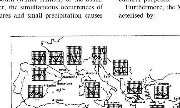
perature associated to annual rainfall in winter. Despite the apparent uniformity of the Mediter-ranean climate, a more detailed analysis shows great differences. The dry season duration (Fig. 1) clearly illustrates that, while the South is
charac-terised by a long dry season, averaging \7
months without any precipitation, in the North-ern part, the dry season is relatively limited and 1. Introduction
The Mediterranean climate is characterised by a hot and dry season in summer and a mild
tem-* Corresponding author. Tel.:+39-080-5475026; fax:+ 39-080-5475023.
E-mail addresses: [email protected] (G. Rana), [email protected] (N. Katerji).
Fig. 1. Duration of the dry season in the Mediterranean basin (Hamdy and Lacirignola, 1999). does not exceed 2 – 3 months. In addition, the
rainfall and temperature diagrams (Fig. 2) show great differences between the North (autumn rain-fall) and the South (winter rainrain-fall) of the basin. During summer, the simultaneous occurrences of high temperatures and small precipitation causes
high evapotranspiration (Hamdy and Lacirignola, 1999). For these reasons, 75% of the available water in the Mediterranean area is used for agri-cultural purposes.
Furthermore, the Mediterranean region is char-acterised by:
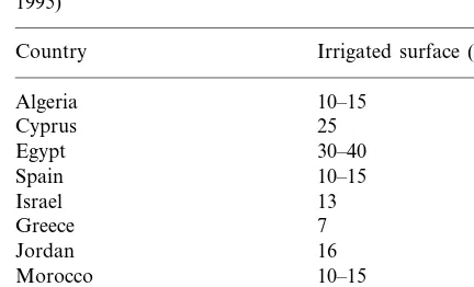
Table 1
Estimation of the percentage of irrigated soils affected by salinity in several Mediterranean countries (Hamdy et al., 1995)
Moreover, semi-arid and, mostly, arid climates have a great impact on crop growth in condition-ing yield and product quality. Under these weather conditions, rainfed crops and agricultural fields with limited water resources are often sub-mitted to water stress. Thus, it becomes funda-mental to know the exact losses of water by evapotranspiration (i.e. actual evapotranspiration) and the crop water status and its influence on production.
Actual crop ET can be measured (directly or indirectly) or estimated. For example, for research purposes in plant eco-physiology, ET must be precisely measured, while for farm irrigation man-agement it can be estimated. The lower the degree of accuracy in the estimation, the greater will be the water waste by incorrect management of irrigation.
In this paper, we review the most important methods of measuring and estimating actual ET, at plot scale (e.g. at farm level), giving, for each method, the problems, limits and advantages for their use in a field under the Mediterranean cli-mate. This summary cannot be, of course, an exhaustive and complete review of all the existing ET methods; in fact, we will focus attention on the most known and diffuse methods in the inter-national research community, paying particular attention to those used in agricultural research.
The scaling up of ET from plot scale to re-gional scale requires specific methods and tech-niques and, therefore, will not be treated in this paper.
2. Measurement and estimation
There is a great variety of methods for measur-ing ET; some methods are more suitable than others for accuracy or cost or are particularly suitable for given space and time scales. For several applications, ET needs to be predicted, so it must be estimated by model.
It is convenient to discuss the methods of deter-mining ET in considering separately the measure-ment and modelling aspects.
Water scarcity in the South: The water
availability in the Southern and Eastern coun-tries of the Mediterranean basin is below the
first needs (1000 m3 per capita per year) and
prospects for the future indicate more severe difficulties (Hamdy and Lacirignola, 1999).
The need to increase the irrigated surfaces
be-cause of the population increasing: The
Med-iterranean population increased by 67%
between 1950 and 1985.
Soil pollution: Nowadays, the problem of
salinity affects 7 – 40% of the irrigated surface of several Mediterranean countries (Table 1). Therefore, accurate determination of irrigation water supply is necessary for sustainable develop-ment and environdevelop-mentally sound water manage-ment. This goal is far from achievement, in fact
the irrigation efficiency is now :45% of the
water supply and one half of this inefficiency could be attributed to bad estimates of crops water requirements (FAO, 1994).
In general, a ‘measurement’ of a physical parameter is a quantification of an attribute of the material under investigation, directed to the an-swering of a specific question in an experiment (Kempthorne and Allmaras, 1986). The quantifi-cation implies a sequence of operations or steps that yields the resultant measurement. Conven-tionally, if the value of the parameter is quantified by the use of an instrument, it is ‘directly’ mea-sured and when it is found by means of a relation-ship among parameters, it is ‘indirectly’ measured (Sette, 1977).
The methods of measuring ET should be di-vided into different categories, since they have been developed to fulfil very different objectives.
One set of methods are primarily intended to quantify the evaporation over a long period, from weeks to months and growth season. Another set of methods has been developed to understand the process governing the transfer of energy and mat-ter between the surface and atmosphere. The last set of methods is used to study the water relations of individual plants or part of plants. Therefore, following Rose and Sharma (1984), it is conve-nient, when discussing the ET measurement, to place the variety of methods in groups, where the main approach or method depends on concepts from hydrology, micrometeorology and plant physiology, as follow:
ET measurement
Hydrological approaches (1) Soil water balance (2) Weighing lysimeters
Micrometeorological approaches (3) Energy balance and Bowen ratio (4) Aerodynamic method
(5) Eddy covariance
Plant physiology approaches (6) Sap flow method
(7) Chambers system
A physical parameter can be considered as ‘es-timable’ if it is expressed by a model. The objec-tive of ET modelling can vary from the provision of a management tool for irrigation design, to the provision of a framework for either detailed un-derstanding of a system or to interpret experimen-tal results. To meet these requirements, it is more convenient to use methods with a sound physical
basis, but often the available data only allow the use of either empirical or statistical approaches. Thus, to discuss the ET modelling, it is convenient to divide the ET models as follows:
ET estimation
Analytical approach
(8) Penman – Monteith model Empirical approach
(9) Methods based on crop coefficient approach
(10) Methods based on soil water balance modelling.
This categorisation is, of course, far from com-pletion, but can be considered a good trace in a review of ET determination.
3. Actual crop evapotranspiration measurement
The different methods for directly and indi-rectly measuring ET are based on the measure-ment of two classes of factors:
1. The soil water content and the physical char-acteristics of the evapotranspirative surface (height, plant density, canopy roughness, albedo);
2. Climatic variables: solar radiation, wind speed and thermodynamic characteristics of the at-mosphere above the canopy.
In the description of the measurement methods, we will consider as true the hypothesis of ‘conser-vative flux’, i.e. the flux density does not change with the height above the canopy. So that, in a first approximation, we will consider the different factors (belonging to both (a) and (b) classes) as constant in the space considered (the field).
The role of the advective regime on the mea-surement and estimation of ET will be analysed in a separate chapter at the end of the methods presentation.
3.1. Hydrological approaches
3.1.1. Soil water balance
Soil water balance is an indirect method, in fact ET is obtained as a residual term in the water balance equation. This equation is based on the principle of conservation of mass in one dimen-sion applied to the soil, its complete expresdimen-sion is:
P+I+W−ET−R−D=9[DS]0
r (1)
where P is precipitation, I is irrigation, W is
contribution from water table upward, R is
sur-face runoff, D is drainage and DS is soil water
storage in the soil layer, where the roots are active to supply water to the plant (r in m). All the terms are in milimeters per unit time. Soil water storage
between two dates (i and i−1) is:
[DS]0r=[Si−Si−1]0r (2)
with S, the soil water content.
Since it is often very difficult to accurately measure all the terms of Eq. (1), a number of simplifications makes this method unsuitable for precise ET measurements. In fact, irrigation water supply is, in principle, known and precipitation can be measured by rain gauges, but all the other terms need to be measured or, at least, estimated. The soil water balance method is applicable to
small plots (:10 m2
) or to a large catchment
(:10 km2); it may cover periods ranging from a
week to a year.
Often, for operational application, the soil wa-ter balance Eq. (1) is expressed in its simplified form:
P+I=ET9[DS]0
r (3)
The simplifications introduced in Eq. (3) could be critical if applied in dry environments. In arid and semi-arid areas with very small slopes, runoff
term R could be neglected (e.g. Holmes, 1984)
but, actually, it depends on the occurrence and characteristics of precipitation (amount, duration
and intensity) and can only be neglected for a particular type of soil (Jensen et al., 1990), i.e. coarse (sand and loamy sand) and moderately coarse (sandy loam).
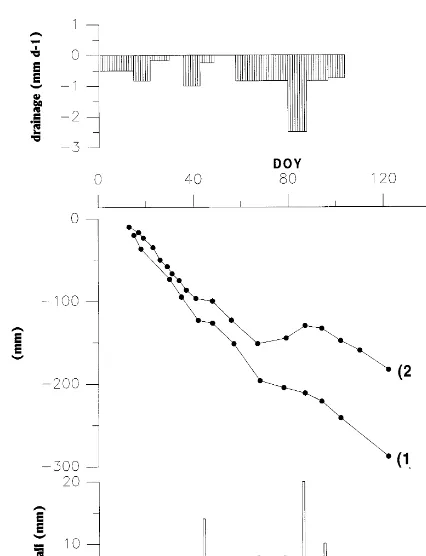
Drainage (D) is the most unknown of Eq. (1).
Some researchers suggest that it can be neglected in dry regions (e.g. Holmes, 1984), but actually it depends on the soil depth, slope, permeability and surface storage (Jensen et al., 1990; Parkes and Li Yuanhua, 1996) and needs to be checked in each particular case (Brutsaert, 1982), depending also on the climate and weather (Katerji et al., 1984). In some situations it is so important that its direct measurement can be used to estimate evapotran-spiration on a weekly or greater scale (for an extensive review see Allen et al. (1991)). More-over, Katerji et al. (1984) demonstrated that it is not simple to establish if the water deep flow can be neglected, in fact it can be a non-negligible fraction of the water balance both in dry and humid seasons and at different time scale. In general, at daily scale it can be neglected if the water supply (Pand/orI) does not exceed the soil water capacity (Holmes, 1984; Lhomme and Katerji, 1991).
In arid regions, the terms W and DS could
show problems of correct evaluation. In fact, if the soil system is closed (i.e. shallow soils or soils
with a very deep water table), W can be
consid-ered negligible and DS can be easily determined.
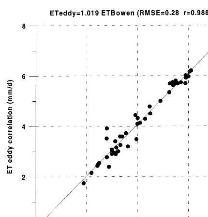
In this case, the simplified soil water balance works well, as shown in Fig. 3, where ET mea-sured by Eq. (3) is compared with a reference method (Bowen ratio). The data are relative to a maize crop grown in a Mediterranean region (Southern Italy) and soil water storage is mea-sured by TDR and the gravimetric method.
Vice versa, if the system is open (deep soils or
soils with a surfacial water table), W cannot be
neglected and DS is difficult to measure exactly,
so that the simplified form of the soil water balance does not work well. This inaccuracy was well demonstrated by Katerji et al. (1984). In fact,
they showed that during humid seasons, W and
DS are of the same order, while during dry
sea-sons, W can reach 30% of cumulated seasonal
Soil water content needs to be measured accu-rately and over an adequate depth. It can be measured by a wide number of methods (an ex-tensive review can be found in Stafford (1988) and Phene et al. (1990)). Three methods are the most important: gravimetric sampling, neutron scatter-ing and electrical resistance.
The gravimetric method remains the most widely used, particularly by technicians and con-sultants; it is well developed at research level and also for irrigation management purposes. It is simple to apply but it can be used only for large time scale (weekly or greater).
Neutron probe remains a useful tool at research level only and its performance has not been
well-established in arid environments. In fact, Payne and Bruck (1996), for example, stated that neu-tron probe tends to lose accuracy under the arid climate of Sahelian Africa, mostly near the sur-face, wetting fronts and textural discontinuities; conversely, Evett and Steiner (1995) found very good results in a wide range of situations.
Fur-thermore, neutron probe poses particularly
difficult and regulatory problems in developing countries.
Electrical resistance matrix type sensors are the least expensive (gravimetry is cheaper) and can be readily used for automatic irrigation control sys-tems (Phene and Howell, 1984; Phene et al., 1989, among many others), but they are not very
Fig. 4. Water balance component for a lucerne crop grown in a deep silt soil; (1) cumulative difference between rainfall and actual evapotranspiration since an initial date; and (2) varia-tion of the total water content in the 0 – 170 cm upper layer of the soil since the same initial date (Katerji et al., 1984).
and hourly scale.
Problems can be encountered in clay soils when the soil moisture is measured by means of probes (neutron scattering, electrical resistance or TDR). In fact, clay soils submitted to an arid climate (i.e. at low moisture content) crack where they are not adequately irrigated (e.g. Diestel, 1993); the deep cracks do not allow suitable contact between soil and probes (Haverkamp et al., 1984a,b) and the reading of the soil moisture can be affected by large errors (Bronswijk et al., 1995).
3.1.2. Weighing lysimeters
Weighing lysimeters have been developed to give a direct measurement of the term ET in Eq. (1). Historically, they have always been consid-ered as a suitable tool to correctly measure evapo-transpiration (Tanner, 1967; Aboukhaled et al., 1982).
In general, it is a device, a tank or container, to define the water movement across a boundary; actually, only a ‘weighing lysimeter’ can deter-mine ET directly by the mass balance of the water as contrasted to non-weighing lysimeter, which indirectly determines ET by volume balance (Howell et al., 1991).
Weighing lysimeters placed in the field contains soil cultivated as the field around it, the sensor is a balance able to measure the weight variation due to ET, often this variation is measured by means of an electronic sensor (i.e. load cell). Under temperate climate, they are able to mea-sure ET at a daily scale with an accuracy of
\10% (Perrier et al., 1974; Klocke et al., 1985b
among others) and at an hourly scale with an accuracy of 10 – 20% (Pruitt and Lourence, 1985; Allen et al., 1991).
However, the weighing lysimeter data are not always representative of conditions of the whole field but, in several situations, they represent only the ET of just one point in the field (Grebet and Cuenca, 1991).
Besides the soil, height and vegetation density differences between the lysimeter and outside veg-etation can severely affect ET measurements. In this case, both aerodynamic and radiative trans-fers to the lysimeter canopy are increasing. If the lysimeter surface and its close area are surrounded rate in estimating actual ET in soil water
deple-tion condideple-tions (see, e.g. Bausch and Bernard, 1996).
The accuracy of soil water balance strongly depends on time and space scales of actual soil moisture measurements (Burrough, 1989) and on
the representativeness of the soil sampling
by drier vegetation or bare soil, an oasis effect occurs. Net radiation in excess of latent heat is converted in sensible heat that is advected toward the lysimeter, resulting in net supply of energy to the lysimeter vegetation. All these previously de-scribed problems cause an increase of ET relative to the surrounding crop. This overestimation of ET could be particularly important under a high radiative climate, as in the Mediterranean region. Furthermore, environmental problems can af-fect measurements of ET with lysimeters (for a review see Allen et al. 1991). One of the most common errors made is the incorrect estimation of an evaporating area of a lysimeter. In fact, this area is calculated by the inner dimensions of the container rather than the true vegetative area, which can be greater than the lysimeter surface when the vegetation from both inside and outside the lysimeter reaches across the rim. This error
could be :20%.
The lysimeter rim can also influence ET mea-surements. One of the most important effects, mainly in arid environments, is the heating of the metallic rim by radiation resulting in microadvec-tion of sensible heat into the lysimeter canopy. Moreover, if the lysimeter rims are too tall rela-tive to crop, the wind is shielded and the radiarela-tive energy balance is modified due to the reflection of solar radiation by the inner wall of the rim to-ward the crop.
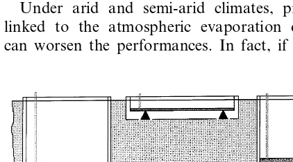
Under arid and semi-arid climates, problems linked to the atmospheric evaporation demand can worsen the performances. In fact, if the soil
inside lysimeters has deep cracks (often along the border in contact with the soil), the water evapo-ration continues from the deepest layers, so that lysimeter can overestimate ET in these periods and underestimate ET in the following periods, when the water depletion inside is greater than that in the field, due to water stress condition of inner plants (Jensen et al., 1990). Conversely, irrigation and rainfall infiltrate into these cracks; this, along with lack of root extraction of water, causes the soil within the lysimeters to be much wetter than the surrounding field soil (Klocke et al., 1991).
Furthermore, the weighing lysimeter is limited in depth in order to make possible the weighing of the soil – plants system; this limitation adds new problems for its use in Mediterranean regions. In fact, it does not take into account the effects of the deeper water fluxes (capillary rising) on crop, which can be very important in water stress peri-ods. Moreover, in areas with deep soil, the weigh-ing lysimeter does not take into account the effects of the total soil available on the plant growth. In this case, i.e. very deep soils, the representativeness of the lysimeter becomes a very difficult technical problem, due to the excessive weight of the system soil – tank – plants. In Fig. 5, three kinds of lysimeter are shown: since the total
available water of nearby soil is :260 mm, only
the first one is well representative of the actual field, but in this case the weight of the system soil – tank is very high (12 t).
3.2. Micrometeorological approaches
From the energetic point of view, evapotranspi-ration can be considered as the energy employed for transporting water from inner leaves and plant organs to the atmosphere as vapour. In this case it is called ‘latent heat ’ (lE, withl, latent heat of vaporisation) and it is measured as energy flux density (W m−2).
We shall describe in the following sections the main methods based on physical or meteorologi-cal principles, by which the latent heat flux can be measured. Three techniques will be analysed: the energy balance and Bowen ratio, the aerodynamic method and the eddy covariance. In general, all Fig. 5. Three kinds of weighing lysimeter:S is surface,Vis
these techniques require accurate measurements of meteorological parameters on small temporal scale (1 h or less). Due to the conservative hy-pothesis of all the flux density above the crop, they can be applied only in large flat areas with uniform vegetation. There are many situations of practical interest where they cannot be used, mostly in the Mediterranean regions. For exam-ple, mixed plant communities, hilly terrain and small plots.
Much care must be taken to analyse local and regional advection under arid conditions (Prueger et al., 1996) and, eventually, to introduce correc-tions to the measured fluxes (see the section on advection).
3.2.1. The energy balance and Bowen ratio method
The latent heat flux can be obtained from mea-surements of the energy budget of the surface
covered with an active growing crop. In fact, lE
represents the major used part of available energy due to the radiation balance. All the energy in-volved in the evapotranspiration phenomenon must satisfy the closure of the energy balance:
Rn−G=H+lE (4)
where we neglect advective processes and where
Rn(W m
−2), net radiation and
G (W m−2), soil
heat flux, are directly measurable by net-radiome-ters and soil heat flux plates, respectively (for an extensive review of environmental
instrumenta-tion see Fritschen and Gay (1979)); and H is the
sensible heat flux density (W m−2).
We define the Bowen ratio b=H/lE, so Eq.
(4) can be rearranged to give
lE=Rn−G
1+b (5)
bcan be measured by the ratio of the air
temper-ature difference between two levels (DT) and the
vapour pressure difference (De), with e (kPa) air vapour pressure, measured at the same two levels:
b=gDT
De (6)
The Bowen ratio is an indirect method, its accuracy has been analysed by many authors (e.g.
Fuchs and Tanner, 1970; Sinclair et al., 1975; Revheim and Jordan, 1976) and can be estimated to be within 10% of the measured value. The Bowen ratio method has been widely studied in a variety of field conditions and it has been proven a standard very accurate method in semi-arid environments (e.g. Dugas et al., 1991; Frangi et al., 1996; Zhao et al., 1996) and for tall crops also (Cellier and Brunet, 1992; Rana and Katerji, 1996).
As previously stated, under arid climates the
crops can experience water stress. In this caseDT
can be quite high but Deis very low; so that it is very important to have highly accurate measure-ments of air vapour pressure (Angus and Watts, 1984). The usual and simplest way is to use differ-ential psychrometry; to meet the requirements of accuracy, for continuous recording, one has to keep the bulbs wet and clean (Fritschen and Gay, 1979). Furthermore, the used thermometers have to be well calibrated, in order to detect tempera-ture differences of 0.05 – 0.2°C; accuracy can be sensibly improved by fluctuating the psycrometric system (Webb, 1960; Gay, 1988; Fritschen and Simpson, 1989).
Recently, improvements have been obtained by using: (i) just one hygrometer that measures alter-natively the humidity of air pumped from two levels (Cellier and Olioso, 1993); (ii) a single cooled mirror dew point hygrometer (some such instruments are briefly described in Dugas et al.,
(1991)); and (iii) spatial averaging systems
(Bausch and Bernard, 1992). In any case, techni-cal problems remain in the hygrometers for the measurement of air humidity in arid regions, espe-cially during water stress periods, when its value is usually very low.
3.2.2. The aerodynamic method
If we assume that a flux density can be related to the gradient of the concentration in the atmo-spheric surface layer (ASL), the latent heat flux by the aerodynamic technique can be determined
di-rectly by means of the scaling factors u* and q*,
with q specific air humidity (kg kg−1), (see e.g.
Grant, 1975; Saugier and Ripley, 1978):
herer is density of air (kg m−3) and the friction
wherek=0.41 is the von Karman constant,d(m)
is the zero plane displacement height,z0(m) is the
roughness length of the surface and Cm is the
stability correction function for momentum
trans-port.q* is determined similarly from the humidity
profile measurement:
where q0 is the air humidity extrapolated at z=
d+z0andC6is the correction function for latent
heat transport.
The calculation of stability functions is made by iterative processes (e.g. Pieri and Fuchs, 1990); users who did not take stability corrections into account have been criticised (Tanner, 1963; Per-rier et al., 1974). The problem of taking into account the atmospheric stability is particularly important in arid environments. In fact, the cou-pling of dry soil and rapid warming or cooling up of air at contact with the earth surface (vegetation or bare soil) leads to extreme conditions of strong stability and instability, with sudden passage from a regime to the opposite one.
The major difficulty with this technique is the correct measurement of the vapour pressure at different heights above the crop. For this reason
lE can be derived indirectly by the energy balance
Eq. (4) if the sensible heat flux is determined by the flux-gradient relation:
H= −rcpu*T* (10)
where T* is deduced by the air temperature
profile:
where T0 is the temperature extrapolated at z=
d+z0 and Ch is the correction function for the
heat transport.
Under this form, the main advantage of the aerodynamic technique consists in avoiding hu-midity measurements. Nevertheless, the accuracy depends on the number of measurement levels of wind speed and temperature profiles. In fact, Eq. (8) and Eq. (11) require at least three or four levels (Webb, 1965), but accuracy is improved when several levels are used (Legg et al., 1981; Wieringa, 1993). When the stability correction functions of Dyer and Hicks (1970) and Paulson (1970) are used, this method gives good results (Grant, 1975; Pieri and Fuchs, 1990).
A simplified version of the method has been proposed by Itier (1980, 1981) and Riou (1982),
based on the measurement of Du and DT, i.e.
wind speed and temperature at two levels only. This method was successfully used to measure actual evapotranspiration of soybean grown in a region of Southern Italy (Rana et al., 1990).
The aerodynamic method does not work with enough accuracy on tall crops, neither in its com-plete form (Garratt, 1978; Thom et al., 1975) nor in its simplified form (Rana and Katerji, 1996). Correction for making this method applicable for tall crops was attempted by Cellier and Brunet (1992).
3.2.3. The eddy co6ariance
The transport of scalar (vapour, heat, CO2) and
vectorial amounts (i.e. momentum) in the low atmosphere in contact with the canopies is mostly governed by air turbulence. The first complete scientific contributions to this topic were given by Dyer (1961) and Hicks (1970); for extensive de-tails of the theory see, for example, Stull (1988).
When certain assumptions are valid, theory pre-dicts that fluxes from the surface can be measured correlating the vertical wind fluctuations from the
mean (w%) with the fluctuations from the mean in
concentration of the transported admixture. So that for latent heat, we can write the following
covariance of vertical wind speed (m s−1) and
vapour density (q% in g m−3):
lE=lw%q% (12)
By making measurements of the instantaneous
fluctuations of vertical wind speed w% and of
contribution from all the significant sizes of eddy and summing their product over an hourly time scale (from 15 min to 1 h), Eq. (12) gives directly the actual crop evapotranspiration.
A representative fetch is required; fetch to height ratios of 100 are usually considered ade-quate but longer fetches are desirable (Wieringa, 1993). The distribution of eddy size contributing to vertical transport creates a range of frequencies important to eddy correlation measurements (for a brief review of the method requirements, see Tanner et al. (1985)). The sensors must suffi-ciently respond to measure the frequencies at the high end of the range, while covariance averaging time must be long enough to include frequencies at the low end (Kaimal et al., 1972; McBean, 1972).
To measure ET directly by this method, vertical wind fluctuations have to be measured and ac-quired contemporary to the vapour density. The first one can be measured by sonic anemometer, the second by fast response hygrometer; both have to be acquired at a typical frequency of 10 – 20 Hz. The Krypton-type fast hygrometers perform well in the field, but they are expensive and very delicate, so they need particular mainte-nance. In fact, the commercial fast hygrometers can be severely damaged if moistened, therefore they can only be installed during the day period, which makes it difficult to use this instrument continuously for a period longer than a few days. Furthermore, errors in eddy covariance method can be due not only to possible deviations from the theoretical assumptions, but also to problems of the sensors configuration and meteorological characteristics (Foken and Wichura, 1996).
One important hypothesis to be verified is that time series must be stationary at the scale of the averaging period, which requires some kind of detrending of the original turbulent signals, like linear detrending or more complex high-pass filtering (Kaimal and Finningan, 1994).
Other known problems are due to the geometri-cal configuration of the sensors. A distortion of the flow can be caused by the sensor arrangement of the anemometer itself and other sensors. The spatial separation between the sonic anemometer and the hygrometer can cause lack of covariance
between the wind speed and the humidity fluctua-tions. In fact, the typical distance between the measuring path of the vertical wind fluctuation and the hygrometer is 30 – 40 cm, this spacing acts like a lower-pass filtering process on the measured signals and must be corrected (Foken and Wichura, 1996).
An important aspect to be considered is the density correction (Webb et al., 1980), this correc-tion is particularly important in semi-arid envi-ronments, in fact it is proportional to the sensible heat flux and may be quite large for high Bowen ratio (Villalobos, 1997).
To avoid some of the above problems linked to
the humidity fluctuations measurements, lE can
be obtained indirectly as residue of the energy budget Eq. (4) if the sensible heat flux is expressed by:
H=rcpw%T% (13)
where cp (J kg−1 C−1) is the specific heat and
density of air. The wind speed and temperature fluctuations are measured by means of sonic anemometer and fast response thermometer, respectively.
Despite problems linked to the correct manage-ment of the sensors and data remain, this method has very good performances both at hourly and daily scale, also in semi-arid environments. In Fig. 6, the comparison between ET measured by this method and Bowen ratio method, at daily scale, is shown for a tall crop (sweet sorghum) grown in Southern Italy.
In conclusion, the use of eddy covariance for latent or sensible heat flux is still a useful tool only at research level, even if the recent develop-ment of robust sensors could permit in the future its practical application in arid regions.
3.3. Plant physiology approaches
Fig. 6. Comparison between ET measured by eddy covariance for sensible heat flux and ET measured by Bowen ratio method, at daily scale, on sweet sorghum grown in Southern Italy (Rana and Katerji, 1996).
stem from the heater element. The difference be-tween the heat input and these losses is assumed to be dissipated by convection with the sap flow up the stem and may be directly related to water
flow (Kjelgaard et al., 1997). The mass flow rateF
(g t−1) is expressed by the relationship:
F=Qh−Qv−Qr
cw·dT
(14)
where Qh is input heat, Qv is vertical conductive
heat, Qr is radial heat loss to environment, cw (J
g−1
K−1
) is specific heat of water and dT is the
temperature difference between the upstream and downstream thermocouples. With the commercial instrumentation, the mass flow rate per plant can be measured at hourly scale.
The micro-engineering problems of the heat emitters and detectors discussed by Cohen et al. (1981) were recently overcome by Kjelgaard et al. (1997), by using constant heat input instead of variable heat input and using surface-mounted thermocouples instead of the inserted ones. These gauges do not disturb the plant root medium but there is still biometric difficulty in extrapolating from one or more plants to the canopy. Further-more, in spite of the fact that the heat balance method is more dependent upon the sap flow rate than upon stem anatomy (Zhang and Kirkham, 1995), at low flow rates (often the case in a semi-arid and arid environment when the crops are under water stress) important differences were observed between the sap flow determined by the gauges and plant water losses observed by a refer-ence method (Kjelgaard et al., 1997). The best results are obtained at a daily scale, mostly on trees.
For the sap flow method it is necessary do a scaling up of the transpiration measurement from plant to field scale. This is possible only if the canopy structure and the spatial variability of the plants characteristics (density, height, LAI) are precisely known.
Recently, Grime and Sinclair (1999) reported sources of error for the constant power stem heat balance method when commercial gauges are used. Their analysis demonstrated that measure-ment errors in determining the diurnal pattern of transpiration could be due to the heat storage in 3.3.1. Sap flow method
Sap flow is closely linked to plant transpiration by means of simple accurate models; sap flow can be measured by two basic methods: (i) heat pulse and (ii) heat balance.
In heat pulse method, applied by Cohen et al. (1988) in herbaceous plants, sap flow is estimated by measuring heat velocity, stem area and xylem conductive area. This method seems to be inaccu-rate at a low transpiration inaccu-rate (Cohen et al., 1993); moreover, it needs calibration for every crop species.
the stem and the pattern of ambient temperature. Moreover, the determining of the sheath conduc-tance by the night-time sap flow measurement can be affected by error due to the stem variation during the season.
These errors are highly dependent on operating conditions and can be minimised by following appropriate recommendations.
Problems linked to the death of the fresh tissues around the heated area, due to silicone applica-tion, can be minimised by reducing the period of continuous measurement to 1 – 2 weeks (Wiltshire et al., 1995).
The sap flow method approaches only transpi-ration measurements, neglecting soil evapotranspi-ration. Nevertheless, under the Mediterranean climate evaporation from soil can be a very important fraction (up to 20% of total evapotranspiration) of the soil – plant – atmosphere water budget (Brut-saert, 1982; Klocke et al., 1985a,b).
3.3.2. Chambers system method
The chambers to rapidly measure ET were de-scribed for the first time by Reicosky and Peters (1977). They consist of aluminium conduits cov-ered with Mylar, polyetilene or other plastic or glass films; the air within the chamber was mixed continuously with strategically located fans. The first version was portable (by means of a tractor, for example) and ET rate was calculated by a psychrometer before the chamber was lowered on the plot and 1 min later, as latent heat storage. The volume of the chamber can be easily adapted to a herbaceous field crop and the accuracy was
:10%, compared with weighing lysimeters
(Rei-cosky et al., 1983).
This system was used by Reicosky (1985) to measure, on a daily scale, ET on several different treatments more easily than the weighing lysime-ter, but it is not suitable for long term ET mea-surements. Furthermore, more serious errors may be introduced if chamber results were extrapo-lated over time as well as spatially (Livingston and Hutchinson, 1994).
Under a semi-arid climate, Dugas et al. (1991) demonstrated that portable chambers, equipped with an infrared analyser (BINOS, Inficon Ley-bold-Heraeus, NY) for measuring vapour density
differences in differential mode, are not represen-tative of the field, particularly on its margins, where ET measurements were affected by sur-rounding conditions. Furthermore, the last im-proved version of portable chambers can be very expensive, due to the high costs for key compo-nents (data acquisition system and infra-red analyser) and accurate chamber manufacturing that may require some heavy engineering.
Recent developments of portable chamber sys-tems can be found in Wagner and Reicosky
(1996); here the equipment also provides CO2
measurements, but its complexity and costs limit its use for research to a small temporal scale.
The chambers are also suitable for research studies on orchard crops (Katerji et al., 1994). The most serious problems of almost all chambers are related to the modification of the microclimate during the measurement period. First, the solar radiation balance, since the chambers were de-signed for simultaneous measurement of both
CO2 and water vapour exchanges (Denmead,
1984). These dual requirements are not often com-patible because wall materials are usually selected for high transmission in the short wavelengths,
neglecting the long-wave exchange (:20% of the
incoming short-wave radiation). Second, the air temperature: its rapid increase inside the cham-bers could alter the biological control of leaves transpiration process. Finally, the wind speed: inside the chamber it could be strongly reduced with direct consequences on ET measurement accuracy.
4. Actual crop evapotranspiration modelling
Actual ET can be estimated by means of more or less complex models: the accuracy of ET esti-mation is proportional to the degree of empiri-cism in the used model or sub-models. Thus, we can categorise the ET estimation into three groups of methods:
1. Methods based on analytical modelling of evapotranspiration;
3. Methods based on a soil water balance modelling.
4.1. ET analytical models
One-dimensional equations based on aerody-namic theory and energy balance — for this reason called combination models (Penman, 1948; Monteith, 1965, 1973) — have proved very useful in the actual crop ET estimation, because they take into account both the canopy properties and meteorological conditions (Szeicz and Long, 1969; Black et al., 1970; Szeicz et al., 1973).
The most widely used form of the combination equation, called Penman-Monteith equation, can be expressed under the form (Allen et al., 1989):
lE=DA+rcpVPD/ra
D+g(1+rc/ra)
(15)
In Eq. (15) we can distinguish weather non-para-metric and paranon-para-metric variables:
weather non-parametric variables: A=Rn−G
(W m−2) is available energy,
D (kPa C−1), is
the slope of the saturation vapour pressure versus temperature function, VPD (kPa) is air
vapour pressure deficit and g(kPa C−1
) is the psychrometric constant;
parametric variables:ra (s m−1) is the
aerody-namic resistance and rc (s m
−1) is the bulk
canopy resistance.
All the terms have to be accurately evaluated (Allen, 1996). While the non-parametric data are standard measurable climatic variables, the para-metric data are not directly measurable and they need to be modelled. Indeed, the first one (ra) is
the aerial boundary layer resistance and describes the role of the interface between canopy and atmosphere in the water vapour transfer; the
sec-ond one (rc) is the resistance that the canopy
opposes to the diffusion of water vapour from inner leaves toward the atmosphere and it is influenced by biological, climatological and agro-nomical variables. This model is applied to the whole plant community as if it were a single ‘big leaf’ located at the height of virtual momentum absorption (Thom, 1975).
The degree of empiricism of the Penman – Mon-teith equation (and consequently its success)
mainly depends on the accuracy of the estimation of the canopy resistance (Beven, 1979).
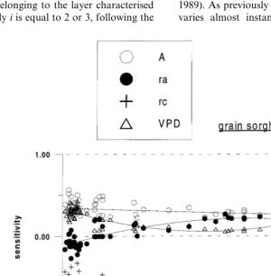
Rana and Katerji (1998) demonstrated that, under a semi-arid climate, the canopy resistance plays the major role, so that its modelling is the most critical point of the Penman – Monteith model to estimate actual crop ET under the Med-iterranean climate. In particular, their sensitivity analysis on Penman – Monteith model showed that: (i) in well-watered conditions,rcmodelling is
sensible to Rnvariations in the case of low crops
(i.e. reference grass) and it is sensible to vapour pressure deficit variations, both in the case of medium (Fig. 7) and tall crops (Fig. 8); (ii) in water stress conditions, rcmodelling is sensible to
the actual crop water status (Figs. 7 and 8).
4.1.1. Methods of determining canopy resistance
One of the most diffuse methods of estimating
rcis that proposed by Szeicz and Long (1969), in
which canopy resistance can be determined as a function of daily mean stomatal resistance of the single leaves (rs) and leaf area index of the leaves
effective in transpiration (LAIeff). These authors
assumed that only the surfacial layer of the canopy participates effectively to the transpira-tion. Usually, such a canopy resistance is assumed to be half the full crop LAI:
rc= rs
LAIeff
(16)
This equation is suggested to be used for refer-ence crop ET (Allen et al., 1989) and it is also used, under light different form, for field crop ET (Steiner et al., 1991; Stannard, 1993; Howell et al., 1995).
Since the spatial and temporal variability of the soil water status (and, consequently, of the plant water status) is very high and the microclimate to which they are exposed is very different (Den-mead, 1984), to obtain sufficiently accurate canopy resistance values by means of this method, it is necessary to realise a great number of mea-surements of stomatal resistance in a brief interval time.
completely solved (Jarvis and McNaughton, 1986; Baldocchi, 1989; Baldocchi et al., 1991; Raupach, 1995); particularly in semi-arid environments (Ste-duto et al., 1997).
An improvement of this estimating method has been proposed by Monteith (1965) and tested and applied by Katerji and Perrier (1985). In this method, the canopy was divided into layers and canopy resistance was estimated starting from stomatal resistance measured layer by layer and weighted with the LAI of each layer. The
expres-sion of the canopy conductance (gc=1/rc) is
given, in this case, by the relationship:
gc=%
i
gci·LAIi (17)
where gci is the stomatal conductance measured
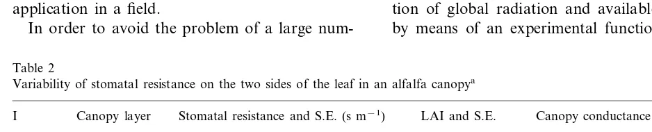
on the leaves belonging to the layer characterised by LAIi. Usuallyiis equal to 2 or 3, following the
crop growth: an example is given in Table 2 for an alfalfa crop divided into three layers. This approach is difficult and hard to carry out, giving
rc values not always accurate. Nevertheless, the
estimation of field crop ET can be acceptable, at least for well-watered crops (Katerji and Perrier, 1985).
The most complete model ofrcshould have the
following general form (Stewart, 1988, 1989; Itier, 1996):
rc=f(LAI,Rg, VPD,T, crop water status) (18)
where Rg is global radiation.
Actually, the better way to evaluate the crop water status is by means of measurements of leaf water potential (Cf) or root-sources abscisic acid
(ABA) (Zhang et al. 1987; Zhang and Davies, 1989). As previously stated, the plant water status varies almost instantaneously, so that to have
Fig. 8. The sensitivity coefficients as function of predawn leaf water potential (PLWP, MPa) for sweet sorghum; for symbols see Fig. 7 (Rana and Katerji, 1998).
acceptable accuracy of the actual crop water
status, a great number of Cf or ABA
measure-ments has to be carried out during the entire day. Hence, this method is not suitable for practical application in a field.
In order to avoid the problem of a large
num-ber of punctual measurements, a numnum-ber of mod-els as expressed by the general relationship Eq. (18), have been developed for dry conditions. For
example, Hatfield (1985) modelled rcin the
func-tion of global radiafunc-tion and available soil water by means of an experimental function. Fuchs et
Table 2
Variability of stomatal resistance on the two sides of the leaf in an alfalfa canopya Stomatal resistance and S.E. (s m−1)
Canopy layer LAI and S.E. Canopy conductance (mm s−1)
I
Lower side Upper side
Top 117929 115929 1.7590.35 30.2
1
Medium 199970
2 5599196 2.190.42 14.3
10449365
3 Bottom 12009420 0.8590.17 1.5
46.0 4.7
Canopy
al. (1987) stated thatrccan be modelled by means
of photosynthetic active radiation (PAR) and soil moisture deficit, but this model is only valid for mild to medium stress. Again, regressive experi-mental functions were used by Jarvis (1976) to
model rcin the function of LAI, Rg, VPD,T and
soil water potential. Unfortunately, all these func-tions need to be locally calibrated per crop and, often, they need also a time calibration, i.e. they are not valid for the whole growth season (Stew-art, 1988).
An original approach to take into account the crop water status to estimate ET by means of Penman – Monteith model was presented by Rana
et al. (1997b), in which rcis modelled as a
func-tion of ‘predawn leaf water potential’, Cb. This
parameter represents the crop water status and it does not need to be measured instantaneously, but just once a day. The application of such a model in semi-arid environments gives quite good
results. Such rcmodel is valid for crops growing
under semi-arid climate (i.e. also for crops under water stress) and needs to be calibrated only ‘per crop’ so that it can be generalised (Rana et al., 1997c). It is possible to use the transpirable soil
water as input of the model instead ofCb, but in
this case the model looses its generality and must be locally calibrated (Rana et al., 1997a).
4.2. ET empirical models
By these methods, the water consumption of crops is estimated as a fraction of the reference evapotranspiration (ET0):
ET=Kc·ET0 (19)
whereKcis the experimentally derived crop
coeffi-cient and ET0 is the maximum
evapotranspira-tion; the latter can be evaluated (i) on a reference crop or (ii) on free water in a pan. The accuracy of such an estimation depends on:
the reference chosen (grass meadow or free
water in a standard pan);
the method used to evaluate reference ET
(measurement or modelling);
the method used to evaluate the crop
coeffi-cient Kc.
Moreover, the data necessary for the
determi-nation of reference evapotranspiration ET0 are
usually collected in standard agrometeorological stations. These stations are usually installed to be representative of the catchment, i.e. an area of several squared kilometres in extension.
4.2.1. ET0 reference crop determination
In this case, ET0 is the water consumed by a
standard crop. In order to make procedures and results comparable world-wide, a well adapted variety of clipped grass has been chosen. It must be 8 – 16 cm high, actively growing and in well-wa-tered conditions, subjected to the same weather as the crop whose water consumption is to be
esti-mated. ET0can be again measured (e.g. by means
of a weighing lysimeter) or estimated. Therefore the comments and observations made for actual
crop ET are still valid for ET0 determination. In
the following, we analysed the more used models of ET0.
A semi-empirical approach to estimate ET0was
proposed by Penman (1956) as:
ET0=
with u2, wind speed measured 2 m above the soil
surface.
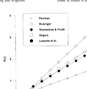
The empiricism of this formula is into the wind
function f(u). Actually, this function is just a
linear regression adjustment to take into account the differences between estimated and observed
ET0 for grass grown in the UK. Therefore, it is a
pressure deficit, which increases going from North to South Europe (Choisnel, 1988).
Today the most used and suggested method to evaluate reference ET is based on the Penman – Monteith model, therefore, having the same prob-lems encountered in actual crop ET estimation
regarding rc modelling.
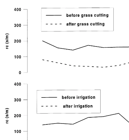
Rana et al. (1994) proposed an ET0 estimated
by means of the Penman – Monteith model, in which canopy resistance is analytically modelled. This model was tested in Mediterranean regions, but it is valid in humid environments too. They demonstrated thatrcvaries with the climate and it
is sensitive to any agronomic practice (irrigation date, grass cutting, phytopathological situation);
in Fig. 10 hourly rcvalues are shown before and
after grass cutting and irrigation.
Recently, Todorovic (1997) proposed a variable canopy resistance, both at hourly and daily scale, modelled in the function of standard
meteorologi-cal parameters. It was shown that ET0 calculated
by the Penman – Monteith model with such a re-sistance works well under different climates.
Several authors proposed an ET0 Penman –
Monteith formula using constant value of rc
(Al-len et al., 1989). Steduto et al. (1996) tested such ET0 estimates with constantrcin several
Mediter-ranean regions. Their results demonstrated that this approach does not have good performances in all the experimental sites.
Other simpler methods to estimate reference crop ET are based on statistical – empirical formu-las (an exhaustive review of these methods can be found in Jensen et al. (1990)). These methods can
Fig. 10. Canopy resistance during a day for a reference grass grown in Southern Italy, (a) before and after grass cutting and (b) before and after irrigation (Rana et al., 1994).
4.2.2. The reference ET0 calculated by the pan
e6aporation
Pan evaporation data can be used to estimate
reference ET, using a simple proportional
relationship:
ET0=Kp·Epan (23)
where Kp is dependent on the type of pan
in-volved, the pan environment in relation to nearby surfaces and the climate. Doorenbos and Pruitt (1977) provided detailed guidelines for using pan
data to estimate reference ET0. In the case of a
pan surrounded by short green grass, Kp ranges
between 0.4 and 0.85. In semi-arid environments
its mean value is :0.7 (Jensen et al., 1990). The
value of Kp to be adopted is strongly dependent
on the upwind fetch and on the local advection.
An attempt to model the pan coefficient,Kphas
been made by Perrier and Hallaire (1979a,b), on the basis of experimental pan data measured in a humid – tropical area (Baldy, 1978). They
ex-pressed Kp in the function of climatic variables
and a coefficient b, the ratio between the
ex-change coefficient of the pan and the wind
func-tion f(u) of the Penman’s formula, as
Kp=
1+a(1−RH)
1+ab(1−RH) (24)
with RH relative air humidity and aa coefficient,
function of air temperature, net radiation and wind speed. This latter coefficient is dependent on be used very easily from a practical point of view,
above all in rural lands. However, their empiri-cism may lead to very inaccurate estimations, as clearly shown by Ibrahim (1996), in arid environ-ments (Table 3).
Table 3
Seasonal reference evapotranspiration (ET0) in 3 years and average percent deviation from the mean value in the north central area of the Nile delta region (Egypt) (Ibrahim, 1996).
Percent deviation from mean value Method Seasonal ET0 Average seasonal ET0(cm)
1979 1980 1981
(a) Blaney–Criddle 63.2 61.81 60.31 61.71 −4.37
66.78 63.20 66.82 65.60 +1.66
(b) Radiation
(c) Modified Penman 62.82 60.60 60.24 61.22 −5.13 81.97
82.92 +27.03
81.35 81.64 (d) Rijtema
49.73 48.00 49.96
(e) Thornthwaite 52.16 −22.59
86.75 80.50
(f) Jensen and Haise 79.41 82.08 +27.20
54.14
56.75 −17.28
(g) Evaporation pan 49.24 53.38
−6.59 60.28
63.47 58.45
(h) Turc 58.93
66.62
Fig. 11. Theoretical curves of pan coefficientKpin function of relative air humidity (a=0.8), b=2 is for humid seasons,
b=2.5 is for medium seasons andb=3 is for dry seasons (Perrier and Hallaire, 1979b).
4.2.3. The crop coefficient Kc
The crop coefficient represents an integration of the effects that distinguish the crop from the
reference ET; many such Kc are reported in the
literature (e.g. Doorenbos and Pruitt, 1977; Allen et al., 1998) usually derived from soil water bal-ance experiments.
Crop coefficient can be improved for estimating
the effects of evaporation from wet soil on Kcon
a daily basis (Wright, 1982). In this case, the crop coefficient can be expressed by the equation:
Kc=Ks·Kcb+Ke (25)
where Ks is a stress reduction coefficient (0}1).
Kcb is the basal crop coefficient (0}1.4) and
represents the ratio of ET and ET0 under
condi-tions when the soil surface is dry, but where the soil water content of the root zone is adequate to sustain full plant transpiration; Ke is a soil water
evaporation coefficient (0}1.4). It can be experi-mentally calculated in the function of soil water
storage, DS and depends on the amount of soil
available to the plants’ roots. In fact, in open soil systems, when the conditions are favourable for
root system development, Ks is almost constant,
also when soil humidity decreases considerably, because of an appreciable contribution of the non-rooted soil layer to the water balance. In closed soil systems (pots, for example) Ks is
vari-able following the soil humidity and it begins to decrease appreciably for values of soil water re-serve :60 – 70% of available soil water to transpi-ration. ThisKsbehaviour is reported in Fig. 12, in
which the ratio of actual to potential ET of a well-irrigated corn crop is reported in the function of the available soil water, for the above men-tioned two conditions (open and closed soils).
In order to avoid the difficulties linked to the available soil water conditions, it is possible to
evaluate Ks by means of the predawn leaf water
potential,Cb. Itier et al. (1992) demonstrated that
this relationship (and Ks as a consequence) has
general validity, since it does not depend on the soil type and site.
The methods to estimate crop coefficients and reference ET have been recently modified by Allen et al. (1994a), Allen et al. (1994b) and Allen et al. (1996).
the site climate and can be considered constant
and =0.8 in arid environment. Fig. 11 shows the
coefficient Kp in the function of RH for three
values of b(b=2, humid seasons;b=2.5,
inter-mediate seasons;b=3, dry seasons).
The crop coefficient plays an essential role in practice (Pereira et al., 1999) and it has been widely used to estimate actual ET for irrigation scheduling purposes. However, it can be subject to serious criticism regarding the meaning and the use of crop coefficient. Besides obvious variations among different crops, empirical crop coefficients were shown to be affected by crop development and weather conditions (De Bruin, 1987). Fur-thermore, Stanghellini et al. (1990) demonstrated that no coefficients should be expected to vary according to the conditions of both climate and crop stage under which they are derived. Moover, these researchers stated that the crop re-quirements based on a same value of the crop coefficient do not have the same accuracy for different months, different seasons, and, above all
at different sites. This inaccuracy of the Kc
ap-proach can be found in the discrepancies between
local calculated Kcand crop coefficients reported
in literature (e.g. Rana et al., 1990; Vasic et al., 1996).
4.2.4. Soil water balance modelling
An exhaustive survey of the most diffuse mod-els for soil water balance can be found in de Jong and Bootsma (1995) and Leenhardt et al. (1995). Two classes of models are generally retained for the simulation of soil water balance: (i) mechanis-tic models and (ii) analogue (or water reservoirs) models.
In the mechanistic approach, the water flux in the soil is controlled by the existence of soil water potential gradients, by means of Darcy’s law and continuity principle. The equations are usually solved by different methods, all involving the splitting of the soil in more or less small layers (de Jong, 1981; Feddes et al., 1988). The difficulties in the application of these models are linked to (i) the accuracy of the used pedo-transfer functions for estimating the water transfer and (ii) the pro-cedures used for estimating the boundary condi-tions of the soil – plant – atmosphere system.
In the analogue approach, the soil is treated as a collection of water reservoirs, filled by rainfall or irrigation and emptied by evapotranspiration and drainage. They can be based on the two following principles (Lhomme and Katerji, 1991):
1. determination of soil water storage DS as
function of the soil and roots depth (e.g. Lhomme and Eldin, 1985; Brisson et al., 1992) 2. the split of soil water in readily transpirable soil water (RTSW) and total TSW (e.g. Fre´teaud et al., 1987). The stress coefficientKs
is supposed to be approximately =1 in the
RTSW range, then it decreases as the water reserve is in the TSW range.
In a previous paragraph we have analysed the difficulties in determining the soil water storage and the evolution ofKsin function of DS,
partic-ularly under a Mediterranean climate. Effectively, Ben Nouna (1995) showed that, in semi-arid re-gions with closed system soils, the water reservoir approach can be very useful in estimating actual
ET only if very accurate measurements of DScan
be realised (Fig. 13).
5. ET evaluation in advection regime
All the previously presented methods to
mea-sure and/or estimate actual crop ET are based on
a fundamental critical hypothesis that the consid-ered systems were conservative, i.e. the profiles of air temperature, water vapour concentration and wind speed are constant along the horizontal axe
X(e.g. Itier and Perrier, 1976; Stull, 1988). In the Mediterranean regions, the scarcity of available water resources leads to irrigated lands in a selective way, with the creation of areas characterised by strong discontinuity of water va-pour concentration at surface level, also for simi-lar crops. The air thermodynamic characteristics are strongly influenced by the surface conditions, so that the air passing from a dry field toward an irrigated field is cooled as well as its humidity increases. Hence, near the boundary of the irri-gated field, ET rapidly increases, then slowly de-creases along the wind direction following the thermodynamic characteristics of the air coupled with the vegetation surface.
In general, the latent heat flux density measured or estimated in one point of the plot is, actually, the sum of two terms: (i) a term translating the equilibrium between the evaporative demand of the air determined by the Penman model and crop water conditions; (ii) an additional flux, more or less important, depending on the lateral transfer of energy by advection. From an energetic point of view, latent best flux depends on the modifica-tions of the vapour and thermal characteristics of the air passing through the considered surface.
The theoretical studies on local advection (Philip 1959; Taylor, 1970; Itier and Perrier, 1976; Itier et al., 1994) showed that the advective flux
(Fa) depends on: (i) the fetch F (m); (ii) the
roughness length of the crop,z0(m); (iii) the wind
speed through the friction velocity u* (m s−1);
and (iv) the temperature difference between the
dry and irrigated fields, DT (°C).
From the operational point of view such a situation in which an advection regime is verified leads to two main consequences:
1. In order to have a correct representativeness of ET, it is necessary to correct a posteriori the evapotranspiration measured by means of weighing lysimeters, soil water balance, sap flow method and chambers system method when the fetch is not large enough to avoid
advection effects. A possible simple correction was proposed by Itier et al. (1978) as:
Fa=360·u*·DT 6
z0/F (26)
This correction can be of 1 – 2 mm per day for temperature differences between dry and irri-gated field of 5 – 10°C (Itier et al., 1978). 2. The micrometeorological methods must be
ap-plied in order to make the measurements in-side the equilibrium fully adapted boundary layer. The fetch value assuring an acceptable adapted layer for micrometeorological is re-ported by Wieringa, (1993) as:
F$2z0
where zis the height of the top sensor.
Regarding the Bowen ratio method, it is well known that it can underestimate ET under strong regional advective conditions (Blad and Rosen-berg, 1974). This implies an extensive fetch in the upwind direction for the air flowing over the surface of at least 100 times the maximum height of measurements, but Heilman et al. (1989) demonstrated that the Bowen ratio method can be successfully applied up to fetch-to-height ratios as low as 20:1.
6. Conclusions
In Mediterranean areas submitted to arid and semi-arid climates, ET ranges over a large interval depending on water regimes (irrigated or non-irri-gated fields). Among the other weather variables, air temperature and humidity experience a large gap between night and day and between winter and summer; the wind is very variable moving from the coast to internal areas. So that, in gen-eral, we can state that all the weather variables range in a very large interval of values. Moreover, the variation in one parameter immediately influ-ences all the other variables that are mutually linked. These facts make difficult to correctly evaluate the crop actual evapotranspiration.
Table 4
Classification by space and time of ET methods to measure or model actual evapotranspiration, adapted by Stewart (1984)
Hour Day Month
Minute Growth season Year
Catchment ---Crop coefficient
method---Uniform area — Micrometeorological method-- ---Crop coefficient method---Soil water balance---Soil water balance with TDR---Penman–Monteith
model---Group of plants ---Weighting lysimeter; chambers system---Sap
---Sap flow---Plant
environments. Some methods are more suitable than others in terms of convenience, accuracy or cost for the measurement of ET at a particular spatial and over a particular time scale. In Table 4 the classification of the presented ET methods by space and time scale is shown.
We tried to give, for each method, the advantages and disadvantages for their use in the Mediter-ranean regions; the summary of this analysis for the measurement methods is reported in Table 5.
In summary, two major observations are possible:
Table 5
Summary of the advantages and disadvantages of the ET measurement methods Disadvantages Advantages
Measurement method
Soil water balance Soil moisture simple to be evaluated with Large spatial variability
gravimetric method Difficult to be applied when the drainage and Not expensive if the gravimetric method is used capillary rising are important
Difficult to measure soil moisture in cracked soils
Direct method Fixed
Weighing lysimeter
Difficult maintenance
It could be not representative of the plot area Expensive
Difficult to have correct measurement of the wet Simple sensors to be installed
Energy balance/
temperature if psychrometers are used Suitable also for tall crops
Bowen ratio
The sensors need to be inverted to reduce bias It can be also used when the fetch is 20:1
Difficult maintenance Not very expensive if psychrometers are used
Aerodynamic Simple sensors to be installed It needs to be corrected for the stability Not suitable for tall crops
It does not need humidity measurements Not very expensive
Delicate sensors Eddy covariance Direct method with fast hygrometer
Difficult software for data acquisition Hygrometer very delicate expensive Difficult scaling-up
Suitable for small plots Sap flow
It takes into account the variability among plants The gauges need to be deplaced every 1–2 weeks The soil evaporation is neglected
Chambers method Suitable for small plots It modifies the microclimate Difficult scaling-up It can be used also for detecting emissions of
1. The ET measurement methods are based on concepts which can be critical under semi-arid and arid environments for several reasons: (i) representativeness (the weighing lysimeter, for example); (ii) instrumentation (air humidity sensors for example); (iii) microclimate (advec-tion regime); and (iv) hypothesis of applicabil-ity (the simplified aerodynamic method for example). Thus, in order to establish the de-gree of accuracy of the obtained ET measure-ment and the validity of a method, it is necessary to consider all these parameters. 2. The estimation methods based on an
analyti-cal approach could be very accurate but, usu-ally, they are not practical enough. The more operational estimation methods (crop
coeffi-cient approach, ET0calculation, water balance
modelling) can be generally affected by very large errors.
Nowadays, a new research trend is being devel-oped in order to integrate these two approaches of actual evapotranspiration estimation. These new models tend to introduce into the analytical approach an acceptable degree of empiricism (Al-len et al., 1989; Rana et al., 1994; Pereira et al., 1999). We think that such methods should be accepted and encouraged in the future, since these approaches can greatly improve the water man-agement at farm level, one of the greatest prob-lems of the Mediterranean countries.
References
Aboukhaled, A., Alfaro, A., Smith, M., 1982. Lysimeters. FAO Irrigation and Drainage Paper No. 39, p.69. Allen, R.G., 1996. Assessing integrity of weather data for use
in reference evapotranspiration estimation. J. Irrig. Drain. Eng. ASCE 122 (2), 97 – 106.
Allen, R.G., Jensen, M.E., Wright, J.L., Burman, R.D., 1989. Operational estimate of reference evapotranspiration. Agron. J. 81, 650 – 662.
Allen, R.G., Howell, T.A., Pruitt, W.O., Walter, I.A., Jensen, M.E. (Eds.), 1991. Lysimeters for evapotranspiration and environmental measurements. Proceedings of the Interna-tional Symposium on Lysimetry, July, 23 – 25, 1991, Hon-olulu, HI, ASCE Publication, p. 444.
Allen, R.G., Smith, M., Perrier, A., Pereira, L.S., 1994a. An update for the definition of reference evapotranspiration. ICID Bull. 43 (2), 1 – 34.
Allen, R.G., Smith, M., Pererea, L.S, Perrier, A., 1994b. An update for the calculation of reference evapotranspiration. ICID Bull. 43 (2), 35 – 92.
Allen, R.G., Smith, M., Pruitt, W.O., Pereira, L.S., 1996. Modification of the FAO crop coefficient approach. In: Camp, C.R., Sadler, E.J., Yoder, R.E. (Eds.), Evapotran-spiration and Irrigation Scheduling. Proceedings of the International Conference, November 3 – 6, San Antonio, TX, pp. 124 – 132.
Allen, R.G., Pereira, L.S., Raes, D., Smith, M., 1998. Crop evapotranspiration. Guidelines for Computing Crop Water Requirements. Irrigation and Drainage Paper No. 56, FAO, Rome, p. 300.
Angus, D.E., Watts, P.J., 1984. Evapotranspiration — how good is the Bowen ratio method? Agric. Water Manag. 8, 133 – 150.
Baldocchi, D.D., 1989. Canopy – atmosphere water vapour exchange: can we scale from leaf to a canopy? In: Estima-tion of Areal EvapotranspiraEstima-tion. IAHS PublicaEstima-tion No. 177, pp. 21 – 41
Baldocchi, D.D., Luxmoore, R.J., Hatfield, J.L., 1991. Dis-cerning the forest from the trees: an essay on scaling canopy stomatal conductance. Agric. For. Meteorol. 54, 197 – 226.
Baldy, C., 1978. Utilisation d’une relation simple entre le bac class A et la formule de Penman pour l’estimation de l’ETP en zone soudano-sahe´lienne. Ann. Agron. 29 (5), 439 – 452. Bausch, W.C., Bernard, T.M., 1992. Spatial averaging Bowen ratio system: description and lysimeter comparison. Trans. ASAE 35 (1), 121 – 128.
Bausch, W.C., Bernard, T.M., 1996. Validity of the Water-mark sensor as a soil moisture measuring device. In: Camp, C.R., Sadler, E.J., Yoder, R.E. (Eds.), Evapotran-spiration and Irrigation Scheduling. Proceedings of the International Conference, November 3 – 6, San Antonio, TX, pp. 933 – 938.
Ben Nouna, B., 1995. Caracte´ristation et mode´lisation du bilan hydrique parcellaire pour une culture de sorgho sucrier. Master Thesis, CIHEAM-IAM Valenzano, Bari, Italy, 112 pp.
Bertuzzi, P., Bruckler, L., Bay, D., Chanzy, A., 1994. Sam-pling strategies for soil water content to estimate evapo-transpiration. Irrig. Sci. 14, 105 – 115.
Beven, K., 1979. A sensitivity analysis of the Penman – Mon-teith actual evapotranspiration estimates. J. Hydrol. 44, 169 – 190.
Black, T.A., Tanner, C.B., Gardner, W.R., 1970. Evapotran-spiration from a snap bean crop. Agron. J. 62, 66 – 69. Blad, B.L., Rosenberg, N.J., 1974. Lysimetric calibration of
the Bowen ratio-energy balance method for evapotranspi-ration estimation in the Central Great Plains. J. Appl. Meteorol. 13, 227 – 236.
Brisson, N., Seguin, B., Bertuzzi, P., 1992. Agrometeorological soil water balance for crop simulation models. Agric. For. Meteorol. 59, 267 – 287.