Volume 26, Number 3, 2011, 325 – 340
MARKET RETURN, VOLATILITY AND TRADING VOLUME
DYNAMICS AFTER ECONOMIC CRISIS
1Bramantyo Djohanputro
PPM School of Management
([email protected]; [email protected])
ABSTRACT
This paper attempts to explore the relationships of return – trading volume and volatil-ity – trading volume. Trading volume may represent a proxy of information, liquidvolatil-ity, and momentum. The up and down of trading volume, therefore, contain certain information that can be extracted by traders to make investment decision. Regressions of market return on its lags, volume, and conditional variance and regressions of volatility on its lags, volume, and conditional variance are employed. Traders may respond positive information differently from negative information. To accommodate such behaviour, threshold autore-gressive conditional heteroskedasticity or TARCH is employed. Using market data of Indonesia Stock Exchange between economic crisis and before sub-prime mortgage crisis (from year 2000 to 2007) indicate the existence of return – volume relationships as well as volatility – return relationships albeit not very strong. There is also an indication that traders respond positive information differently from negative information concerning return movements but there is no indication concerning volatility movements.
Keywords: return, volatility, volume, TARCH
INTRODUCTION
After1 experiencing the economic crisis in 1997 – 1998 in Asia, and especially in Indone-sia, the Indonesian Stock Exchange is ex-pected to be more mature and efficient. There are some factors that support such an expecta-tion. Firstly, the number of companies going public increased significantly, from less than 300 companies before the crisis to more than 400 companies. The increase is more than thirty percent and it is considered to be high. Secondly, the regulator has evolved to become more integrated in managing the capital mar-ket. Bapepam (Badan Pengawas Pasar Mo-dal) or Capital Market Advisory Board ex-tends its scope of authority to become
1 The data available in this paper may be used and distributed to anyone needed.
Bapepam LK (Badan Pengawas Pasar Modal dan Lembaga Keuangan) or Capital Market and Financial Institution Advisory Board. This change is expected to cover more integrated information and monitoring to assure the capital market work efficiently and effectively.
fundamental factors to move and, then, react to the expected movement accordingly.
Investors use trading activities to make investment decisions because they are confi-dent that the trading activities contain material information. The possibility that trading activi-ties contain information is supported by some previous studies. Brown et al. (2009) suggest that trading volume may contain several fac-tors valuable including liquidity, momentum, and information. By scrutinizing trading volume, investors may extract some knowl-edge to make decisions such as buy, hold, sell, and portfolio allocation.
Apart from the possibility that trading ac-tivities represented by trading volume may influence market returns, the activities also potentially affects market volatility. However, the sustainability of volatility depends on whether the trading activities have fundamen-tal information or merely reflect psychological shock. The existence of fundamental informa-tion in the trading activities will affect perma-nent volatility, while psychological shock in the trading activities will only influence vola-tility temporary. This is in accordance with Girard and Omran findings (Girard and Omran, 2009), suggesting that the impact of trading activities on market volatility depends on whether the trading activities derive from expected or unexpected components.
Based on those arguments, the paper aims at exploring the investors’ behaviour on in-vestment decisions, especially on how they behave daily by considering trading volume and its impact on share prices and fluctuation. In other words, this paper focuses the study on the relationships between market returns, mar-ket volatility and aggregate trading volume. It is expected to find information on how inves-tors use the trading volume or volume change or the price movements and the volatility of the market.
This research, then, attempts to answer the following questions. Firstly, how and to what
extent do investors use the trading volume as the sources of information on trading that af-fect returns? Secondly, to what extent are trading volume and volatility important to influence price movements? Thirdly, to what extent does trading volume influence the mar-ket volatility?
To answer those questions, this research employs the following variables. Market daily returns derive as the difference in the loga-rithms of stock index levels. Volatility is gen-erated as the squared daily returns. Trading volume, on the other hand, is represented by several operating variables. Firstly, trading volume is defined as the nominal values of trading. Secondly, trading volume is also rep-resented as the logarithm of trading volume. The use of logarithm is to downsize the figures and, at the same time, to reveal the exponential behaviour of trading volume. Thirdly, trading volume variable is represented as the change in the trading volume.
It is important to note that the relationship between return, volatility and volume is well known already (for example, Sabri, 2004). It is recognized too that the market reaction to volatility is different according to the direction of the volatility. Volatility represents risk, and market risk is considered as one of speculative risks. By definition, speculative risk means that the market movement may affect investors positively if the movement is in favour to the interest of investors, or negatively if the move-ment is against the interest of investors. In some cases, investors react differently to the different risk sides.
Based on the aforementioned arguments, the basic questions to be answered are as fol-lows: firstly, is there any relationship between market return and trading activity after the economic crisis 1998? Secondly, is there any relationship between market volatility and trading activity after the economic crisis 1998? Thirdly, how do traders use conditional vola-tility on the trading activities?
This study indicates that the increase (de-crease) in trading volume or activities encour-ages the increase (decrease) in return. An ac-tive market tends to attract traders into the market to trade causing the price to increase, while lower market activity tends to encourage market price to decrease. In relation to volatility – volume, this study indicates that trading volume still considerably has value on explaining the behaviour of volatility. The magnitude of explanation, however, is quite low. Traders prefer more to employ past vola-tility and behave accordingly than to employ trading volume.
This paper is organized as follows. The first section is introduction. The following section describes previous studies related to return – volume and volatility-volume rela-tionship. This is then followed by the proposed models and hypotheses. The next section elaborates data employed in this study and their analysis. This paper is closed with the conclusion.
PREVIOUS STUDIES
Some studies suggest that market returns and trading volume indicate various factors (Lamoureux and Lastrapes, 1990; Chowdury et al. 1993; Hrazdil, 2009). They focus the study on the relationship between returns and trading volume at market level. Some re-searchers also attempt to explore various trading volume against market return, such as foreign trading against market return and block or large trading volume against market return. The purpose is, basically, to extract the information contained in such a trading type
that may influence investor of a market as a whole. The behaviour of investors, as a result, encourages price or index movements or re-turns.
The argument saying that trading volume matters has been supported by several studies. Some studies focus solely on the volume as a determinant factor of price movement (Kymaz and Girard, 2009; Andersen, 1996; Easley et al. 1996). Trading data reflect the underlying information structure. On days when good news dominates the market, more buys are expected. This eventually encourages higher demand and, hence, price increase. On days with dominant bad news, on the other hand, more sells are expected. This, in turn, encourages the price to move down. Some others employ volume among other factors that influence the price movements. Rompotis (2009), for example, finds that volume to-gether with expenses and risks have relation-ship with price premium and trading activity.
Market trading volume also reflects some proxy, including liquidity, momentum, and information (Brown, 2009). Liquid market, expressed by low trading volume as well as frequency, encourages investors to demand high premium. In other words, they ask for low price, with the expectation that they may be able to sell at high price, to obtain high return. In that sense, the relationship between market return and trading volume is negative.
data (Choi et al. 2009). The magnitude of price change depends on the quality of infor-mation content in the trading volume.
Some researchers propose the adverse selection model of trading (Glosten and Milgrom, 1985; Easly and O’Hara, 1987, 1992). They propose that certain traders bring new information and reveal certain characteristics of transaction. Those informed traders tend to trade on one side. At times when they have good news, they conduct to buy while at times when they have bad news they conduct to sell stocks. They also tend to trade in a large volume to exploit the opportunity or to avoid loss. They do this be-cause they bear costs in processing public in-formation into private inin-formation. Other trad-ers, i.e. non-informed or free ridtrad-ers, tend to trade in small volume of transaction, and trade randomly. They just follow what large traders do.
Some informed traders, however, avoid transacting large trades because they want to keep their private information from free riders (for example, Admati and Pjeiderer, 1988, 1989; Foster and Vismanathan, 1994). In fact, at least there are two ways of hiding private information, i.e. through timing and trading size. Under a timing strategy, informed traders may choose to transact under a low total trans-action volume. Under a size strategy, informed traders may transact on several consecutive days for every single stock. As an alternative, they may buy or sell portfolio, assuming that each portfolio contains small faction of each stock. At the end of the day, the total trading conducted by informed traders is large.
Informed traders continue to trade until all information is reflected in the price, or when the price reaches its equilibrium. However, they may not come to the consensus due to the different interpretation of information. Under this case, price equilibrium may be slow to reach. The wider the interpretation of informa-tion, the wider is the diversity of trading
be-haviour. This will result in another factor, i.e. the width of spread (Copeland, 1977).
The pricing and its forecast may improve gradually depending on the information arrival to the market. The smooth, fast, flow of infor-mation helps market participants to review their knowledge and forecast on every stock. The revision of the stock price will certainly move the market as a whole. Gemmil (1994) suggests the gradual improvement in forecast based on the speed of publication. The earlier information becomes public, the quicker trad-ers learn and adjust the forecast.
Others believe that the relationship takes place between trading volume change against price change. However, this relationship may be complicated because the change in trading volume depends on whether the market move-ment is under selling pressure or buying pres-sure. Selling pressure of trading normally takes place under bearish condition, while buying pressure takes place under bullish con-dition. If trading volume increases due to the large investors willing to sell stocks, the price tends to decrease. This represents the increase of stock supply at the constant or even declin-ing demand. On the other hand, if the traddeclin-ing volume increases because many investors want to buy stocks, the price tends to increase. This represents the significant increase in stock demand while the stock supply is con-stant.
To avoid problem of identifying the rela-tionship between trading volume and price movement on either buying or selling pres-sure, one solution is to identify the existence of the relationship between the absolute of price change against trading volume. The pur-pose is to find whether trading volume encourages price movements whatever the direction of the price movement.
whole. This is also known as asset liquidity. Asset liquidity is represented by trading speed, trading cost or spread, price impact, and trad-ing volume (Amihud and Mendelson, 1991; Brown et al. 2009).
As the two relationships, i.e. return - trad-ing volume and volatility – tradtrad-ing volume, are affected by momentum or timing, it is also known that those relationships may change as the time goes by. There are many factors that influence the dynamics of those relationships, such as the change in regulation, government regime, competition, technology applied to the stock market, etc. This is one reason why some studies employ certain period of time, of conduct a stability test before conducting re-search with a long period data.
RESEARCH METHOD
Assume that a trader is an informed trader. S/he has some choices suitable for him/her. S/he may trade on one stock with large volume, or many stocks with low volume for each stock. S/he also can transact index, stock portfolio. Depending on the type of information, s/he will trade on a certain side, either buy side or sell side. No matter the trade size, his/her, his/her persistence in trading causes the trading volume increases significantly. This model follows the argument that total trading volume matters because the total volume may reflect the information con-tained in each transaction (see Andersen, 1996; Easly et al. 1996).
Following Andersen (1996), a joint de-pendence of return and volume applies on an underlying latent event or information vari-able. In a price discovery process, traders ar-rive to the market sequentially and in a ran-dom, anonymous fashion. This type of infor-mation arrivals induces a dynamic learning process of price discovery or information assimilation phase. When all agents agree on the price, the market goes to the equilibrium direction characterized by uniform valuation and low buy-sell spread. In other words, price
discovery phase is followed by an equilibrium phase. Volume and volatility of stock price are driven by similar mechanism.
Under the aforementioned argument, the proposed hypotheses are based on: market anticipation hypothesis and sequential in-formed trading hypothesis. Under the market anticipation hypothesis, it is argued that the ability of traders to predict future events can be applied to specific firm with market-wide scope. Traders are assumed to acquire ability to collect information that may influence mar-ket movement. As marmar-kets become more globalized, the traders need to collect domestic as well as foreign data of market factors.
There are two possibilities the way traders interpret information: optimistic and pessimis-tic. The interpretations depend on the quality of data and the ability to process the data. The market anticipation hypothesis does not ex-plain how traders extract information from data. Instead, the hypothesis focuses on the argument that the trend of market price is the net impact of the optimistic and pessimistic forecast of all traders. As long as the traders tend to agree their interpretation on data to become information, the market movement tends to be less volatile and, in effect, the price reaches the equilibrium more quickly.
The sequential informed trading hypothe-sis assumes that the ability of traders to extract information from data diverse. This implies that some traders may extract information in advance and move to the market more quickly, while other traders work on the interpretation and forecast. In this case, traders enter the market in different point in time. In addition, every time a trader enters the market, other traders employ this movement as an additional data to be processed to extract private infor-mation.
market in different point in time depending on their attitude toward risk and their own timing. However, there is no chance for them to enter the market prior to the best informed traders. In other words, it is possible for market mak-ers, liquidity tradmak-ers, and free riders to enter the market at same time with the second best informed traders, the third best informed trad-ers, and so on. It is also conclusive to say that the last traders must be one of uninformed traders.
Under those basic hypotheses, the follow-ing are the hypothesis buildfollow-ing for this re-search.
Return–Volume Relationships
Kim et al. (2006) develop a return– volume model from a simple model based on the direct relationship between return and volume (Epps, 1975; Copeland, 1977; Campbell et al. 1993). However, the relation-ship may be in two possibilities: negative or positive relationships between the two vari-ables. Those studies add the quadratic form of trading volume as an independent variable and this gives a positive relationship with market return. However, this relationship does not give significant information to explain such a relationship.
Other studies attempt to exploit the mag-nitude of trading volume against price move-ment. They find that the increase in volume is higher when it is accompanied by the increase in price than by the decrease in price (for example, Epps, 1975; Lakonishok and Smidt, 1986). Other studies attempt to distinguish buying-pressure trading from selling-pressure trading. As expected, price decrease is accom-panied by selling-pressure while price increase is accompanied by buying-pressure (Chan and Lakonishok, 1993; Gemmill, 1994; Keim and Madhavan, 1996)
Based on those arguments, it is important to extract the importance of information con-tained in the past and current trading volume
as well as past returns in relation to price movements.
Hypothesis 1: Past and current market volume are significantly related to cur-rent share price.
The equation becomes as follows:
The variables of the above equations are as follows. Return is the daily market return. It is defined as the change in daily market index, i.e.
extract the information contained in the previ-ous trading days. Some investors, either informed traders or noise traders, may find certain information to follow from the way prices moves. The number of lag very much depends on the speed of those traders obtain information and their capability to bear risk in trading.
logarithm, in this study, is merely to scale down the figure.
Variables Dk represent daily dummy
vari-ables. Because there are five trading days within a week, this study employ four daily dummy variables. These variables are to ex-tract the difference in trading behaviour and characteristics on daily basis.
The last independent variable, i.e. σt or
daily volatility, attempts to extract the impact of daily volatility to return. Together with the equation (2), the volatility may become a source of information explored by traders. They may behave differently in terms of trad-ing decisions in high versus low volatility times.
In addition, equation (2) employ TARCH (Threshold Autoregressive Conditional Hete-roskedasticity) model. This follows previous implementation of ARCH and its variance process (Bierens, 1993; Kim and Schmidt, 1993; Schwaiger, 1995; Kim et al. 2006). The use of TARCH process is to improve the efficiency of the volatility in equation (1). The use of conditional variance, h2, is because conditional variance changes through times and it violates the homeoskedasticity assump-tion. The use of TARCH is to catch the asym-metric effect of information on traders’ be-haviour, i.e. to negative and positive infor-mation. Such differences will be captured by coefficients on equation (2), especially by γt.
Note that the implementation of equation (2) depends on the ability of traders to extract information from variance. As long as they believe the quality of information in the vari-ance, equation (2) will be employed accord-ingly. Furthermore, equation may employ other regressor such as the trading volume. It is because sometimes traders do not only con-cern with the variance based on its past vari-ance but also the trading activity. In this case, an independent variable needs to be added in equation (2).
In relation to the volume–return relation-ships, it is expected that volume positively effects return.
Volatility–Volume Relationship
Some studies support the existence of the volatility-volume relationship (among others: Epps, 1975; Smirlock and Starks, 1988, Amihud and Mendelson, 1991; Blume et al. 1994). Following previous studies, Yen and Chen (2010) attempts to evaluate the relation-ship between volatility and total trading vol-ume. They add open interest as a factor under scrutiny. They tend to agree that trading volume contains noise that increases the volatility of prices. Furthermore, the use of volatility ignores the types of trading pres-sures, i.e. selling and buying-pressures. In either case, the increase in trading volume encourages in the high movement in price or volatility.
Based on the above argument, the second hypothesis is as follows:
Hypothesis 2: Current and past trading volume influence current market vola-tility
The equations to represent this hypothesis are as follows:
t a b Volatility
There are two ways of expressing volatility of daily returns. The first is in terms of absolute value returns. The second is in terms of the squared returns.
The use of past volatility in equation (4) is because traders may behave to previous price fluctuation before considering other variables, such as volume. In this case, one expects bi’s
are significant. The length of the lags depends on how fast traders react to the volatility. One also expects that volume positively influences market volatility.
DATA AND ANALYSIS
As explained in the beginning, this study focuses on the period outside crisis. It is well known that economic crisis hit Indonesia and other countries severely in year 1997. The effect of crisis remained devastating until year 1999. Therefore, it is safe to start the analysis from January 1st 2000. It is also well known that economic crisis hit Indonesia again as the contagion effect of sub-prime mortgage crisis in the United States of America. The crisis started in mid-2008 and strongly influenced most industries and also capital market in Indonesia. For this reason, this study employs December 31st 2007 as the end period. The total data from January 1st 2000 to December 31st 2007 are more than 1,500.
The Jakarta Composite Index and trading volume data are taken from yahoo.com. The Jakarta Composite Index consists of all stocks traded in Indonesia Stock Exchange (previ-ously Jakarta Stock Exchange). The index accommodates the change in stocks registered in those indices (Pinfold and Qiu, 2007). One should be careful in using yahoo.com. It is because the data source only records data with trading activity. For that reason, there are many missing working dates within the period employed. Therefore, the time series is scrutinized line by line and fill in the missing
dates with the data. As a common practice, any missing data are filled with the data from previous day for indices and with zero for trading volume.
This study employs the closing index. It is based on an assumption that all information coming to the market are reflected immedi-ately into the price on the same day. The closing price, therefore, reflected all informa-tion available. Any event taking place over-night is accommodated into next day’s price.
Return – Trading Volume
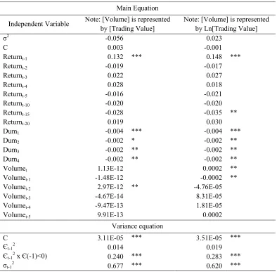
Table 1 shows the results of two main regressions processed with Eviews program with maximum 500 iterations. The first regres-sion results, as shown in columns (2) and (3), applies to the return as the dependent variable and conditional variance, lags of return, and the value of trading volume as regressors. The second regression results, as indicated in col-umns (4) and (5), applies to the return as the dependent variable and conditional variance, lags of return, and the natural logarithm of value of trading volume as regressors. Both regressions use TARCH (1,1) as their variance equations. In relation to the treatment of time series data, this study applies the stationary test to the residuals. Heteroskedasticity and colinearity also apply to the residuals of re-gressions. Some measures used include Durbin-Watson Statistic.
Table 1. The regression of Return on conditional variance, lags, and trading volume with TARCH model for variance equation
Dependent Variable: Return
Main Equation
Independent Variable Note: [Volume] is represented by [Trading Value]
Note: [Volume] is represented by Ln[Trading Value]
σ2
-0.056 0.023
C 0.003 -0.001
Returnt-1 0.132 *** 0.148 ***
Returnt-2 -0.019 -0.017
Returnt-3 0.022 0.027
Returnt-4 0.028 0.018
Returnt-5 -0.016 -0.021
Returnt-10 -0.020 -0.020
Returnt-15 -0.028 -0.035 **
Returnt-20 0.019 0.030
Dum1 -0.004 *** -0.004 ***
Dum2 -0.002 * -0.002 **
Dum3 -0.002 ** -0.002 **
Dum4 -0.002 ** -0.002 **
Volumet 1.13E-12 0.0002 **
Volumet-1 -1.48E-12 -0.0002 **
Volumet-2 2.97E-12 ** -4.76E-05
Volumet-3 -4.67E-14 8.31E-05
Volumet-4 -9.47E-13 1.81E-05
Volumet-5 9.91E-13 0.0002
Variance equation
C 3.11E-05 *** 3.51E-05 ***
Єt-12 0.014 0.019
Єt-12 x Є(-1)<0) 0.240 *** 0.283 ***
σt-12 0.677 *** 0.620 ***
Notes: Significance: *** at 1%, ** at 5%, and * at 10%
Both main regressions indicate that condi-tional variances do not really influence the market returns. This is indicated by the coeffi-cients of σ2 that are not significantly different from zero. This conclusion is supported by the fact that the coefficient of the first regression tends to be negative while the coefficient of the second regression tends to be positive. This inconsistence leads to the inconclusive
relationship between return and conditional variance.
The first lag of return, or Returnt-1,
yester-day’s return is perceived as having certain information that is valuable to be carried to the next day. The positive coefficients indicate that yesterday’s return encourage the move-ment of current return to the same direction. The higher yesterday’s return, the higher is current return.
This kind of amplification must have a limit. Otherwise, there is an error correction or price reversal. It is assumed that price trend reverses after certain period because of noise or mispricing. In other words, price redemp-tion exists to avoid excessive bubble. This is the reason for this study to employ longer lags, i.e. to identify the length of which the return reversal or redemption takes place.
The main regressions shown in Table 1 indicate that price reversal tends to take place at the next two trading days. This is indicated by negative coefficients of Returnt-2 even
though the coefficients are not significantly different from zero. Furthermore, current re-turn also has negative relationship with Re-turnt-5, Returnt-10, and Returnt-15. Those
nega-tive coefficients at least an indication that traders tend to correct price on the basis of prices from the same days of previous week, previous two weeks, and previous three weeks. The main regression that employs Ln[Volumet-i] as an independent variable gives
a stronger message on the traders’ behaviour concerning the price reversal issue. The sig-nificant coefficient (at 5% sigsig-nificant level) is an indication that traders really reverse the price based on the last three weeks price trend.
Both main regressions indicate similar in-formation on how traders behave in trading activities. Hypothesis 1 says that “Past and current market volume are significantly related to current share price”. Column (2) of Table 1 shows that only coefficient of Volumet-2 is
positive and significantly different from zero at 5% significance level. Based on column (4), Volumet has positive coefficient and Volumet-1
has negative coefficient, and both are signifi-cantly different from zero at 5% significant
level. Before those models are chosen, several models with longer lags of volume have been tested. The longest lag is Volumet-20. However,
lags more than a week do not improve statisti-cal indicators, such as maximum likelihood, Akaike information criteria, and Schwarz cri-teria. Instead, longer lags of volume seem to indicate autocorrelation that affect the coeffi-cient of determinant.
The signs of coefficients of Volumet and
Volumet-1 are consistent for both main models.
The coefficients of Volumet are positive, while
the coefficients of Volumet-1 are negative.
Note that Volumet is the trading volume
within a trading day, i.e. from opening until closing transaction. As returns are calculated based on closing price, this means that Volu-met takes place prior to closing price.
Positive and significant coefficient of Volumet quite strongly indicate that the
in-crease (dein-crease) in trading volume or activi-ties encourage the increase (decrease) in re-turn. Under an active market, in which trading volume within a day increases, traders may think that the market is getting more attractive and, as a response, more traders come into the market to transact. This increases buying pres-sure. As a result, prices are pushed to go up and, as a consequence, return increases.
On the other hand, at times when trading activities decrease, traders may think that the market is not attractive any longer. Some trad-ers start to retreat from the market. As a result, buying pressure decreases, prices move more slowly, and the return becomes lower. On one extreme, prices decrease at times when trading activities or trading volume decrease.
The negative coefficients of Volumet-1
overvalued. However, the fact that the coeffi-cient of the first main regression is not signifi-cant may indicate that traders do not always revise their pricing as an effect of trading activities.
The significance level at 5% of the coeffi-cients of Volumet and Volumet-1 leads to
cau-tious interpretation of the return – volume relationships. As mentioned before, the price movements may be different between buying and selling-pressures. In general, the increase in trading volume under buying pressure tends to increase the price while the increase in trading volume under selling pressure tends to push the price down. The period of year 2000 to 2007 is dominated by buying period. It is due to the recovery period of Indonesia econ-omy. For this reason, it is not surprising that trading volume gives positive impact on price movements. In certain period, selling pres-sures may take place. However, these events are less dominant within the period under study than buying pressure events.
It is important to briefly put some note on the variance regression. Both models show that the threshold components of TARCH are positive and different from zero at 1% signifi-cant level. These strong significance levels suggest the existence of different response made by traders on positive from negative information. Traders respond more strongly on negative information than on positive infor-mation for the equal level of inforinfor-mation con-tent.
Volatility–Trading Volume
Tables 2 and 3 show the results of regres-sions of volatility on trading volume. In Table 2, the volatility is represented by absolute value of return or Abs[Return]t. In Table 3, the
volatility is represented by the squared return, or [Returnt]2. In both models, the two types of
volume, i.e. the Value of trading volume, or Volumet, and the natural logarithm of trading
value, or Ln[Volumet], are employed.
Note that there is a very significant differ-ence between models shown in Table 2 and models shown in Table 3. Models in Table 2 employ TARCH model as the variance equa-tion. These models are the best on the basis of several statistical criteria, such as homeoske-dasticity, error stationary, Durbin Watson, maximum likelihood, Akaike information cri-teria, and Schwarz criteria compared to other models that have been tested before choosing these models.
The models also apply Mean-ARCH, by inserting conditional variance as an independ-ent. This is to extract information contained in the error component to the volatility of the market return. Similar to the application to return-volume as explained above, the vari-ance is conditional because this variable may change as the time goes by. This is in relation to the implementation of the variance equa-tion.
This study also evaluates the use of volume variable as a variance regressor. However, the use of such variable does not improve the power of the models. Instead, some statistical indicators are worse than those without variance regressor. As a consequence, TARCH model is implemented without any variance regressor.
Models shown in Table 3, however, do not fit with variance equation model. It is based on several statistical indicators, such as R2 and Durbin Watson statistics. For that reason, con-ditional variance as an independent variable in the main equation and the variance equation are dropped from the model. Other variables, however, are still applicable to the models.
They indicate that past volatilities are posi-tively related to current volatility. If the vola-tility increases (decreases) in the last three days, the current volatility most probably in-creases (dein-creases) too.
The coefficients of Volatilityt-5 and
Vola-tilityt-10 also give an indication on how traders
respond to the past volatility with longer
pe-riod. As shown in Table 2, the significance of the coefficient of Volatilityt-10 shown in
col-umn (2) and (3) are different. In colcol-umn (2), the coefficient is positive and different from zero at 5% significance level. In column (3), on the other hand, the coefficient is positive but not significantly different from zero.
Table 2. The regression result of volatility–volume relationships with Abs[Returnt] as dependent
variable
Main Equation
Independent Variable Note: [Volume] is represented by [Trading Value]
Note: [Volume] is represented by Ln[Trading Value]
σ2
0.612 *** 0.216
C -0.0003 0.004
Abs[Returnt-1] 0.060 ** 0.089 ***
Abs[Returnt-2] 0.089 *** 0.069 **
Abs[Returnt-3] 0.074 *** 0.053 **
Abs[Returnt-4] 0.038 0.011
Abs[Returnt-5] 0.028 0.028
Abs[Returnt-10] 0.044 ** 0.021
Abs[Returnt-15] 0.003 0.034
Abs[Returnt-20] -0.0105 0.006
Dum1 0.002 *** 0.002 ***
Dum2 0.0002 0.0004
Dum3 0.001 ** 0.001 **
Dum4 0.0008 0.001
Volumet 1.02E-12 0.0001
Volumet-1 -1.30E-12 -7.46E-05
Volumet-2 1.87E-12 * -1.03E-05
Volumet-3 -4.76E-13 -6.02E-05
Volumet-4 -4.21E-13 -4.80E-05
Volumet-5 2.44E-13 2.31E-05
Variance equation
C 2.04E-05 *** 9.21E-06 ***
Єt-12 0.150 *** 0.141 ***
Єt-12 x Є(-1)<0) 0.050 -0.024
σt-12 0.600 *** 0.763 ***
Table 3: The regression result of volatility–volume relationships with [Returnt]2 as dependent
variable
Main Equation
Independent Variable Note: [Volume] is represented by [Trading Value]
Note: [Volume] is represented by Ln[Trading Value]
C 7.84E-05 *** 0.0001
[Return2]t-1 0.068 *** 0.059 **
[Return2]t-2 0.149 *** 0.178 ***
[Return2]t-3 0.088 *** 0.095 ***
[Return2]t-4 -0.004 -0.019
[Return2]t-5 0.052 ** 0.064 ***
[Return2]t-10 0.039 * 0.026
[Return2]t-15 -0.006 0.004
[Return2]t-20 -0.031 -0.030
Dum1 0.0001 *** 9.97E-05 ***
Dum2 6.43E-06 -2.69E-06
Dum3 4.16E-05 3.51E-05
Dum4 1.99E-05 1.00E-05
Volumet 3.54E-14 2.63E-06
Volumet-1 -2.78E-14 -1.41E-06
Volumet-2 4.65E-14 5.82E-07
Volumet-3 -1.70E-14 2.29E-07
Volumet-4 -2.59E-14 -2.64E-06
Volumet-5 -9.96E-15 -7.61E-07
Notes: Significance: *** at 1%, ** at 5%, and * at 10%
The coefficients of Volatilityt-5 and
Vola-tilityt-10 shown in Table (3) are different. The
coefficients of Volatilityt-5 are positive and
significantly different from zero at 5% signifi-cant level for the first model and at 1% sig-nificant level. The coefficients of Volatilityt-10
are positive for both models and significantly different from zero at 10% significant level for the first model but not significantly different from zero for the second model.
Those results at least indicate the follow-ing information. Firstly, traders at least con-sider daily volatilities within a week, until 5 lags, to make the decision on transaction. The volatilities within a week positively influence traders on the pricing. The higher (lower) the daily volatilities within a week, the higher
(lower) are the spread of interpretation on price because the price interpretation by trad-ers is more (less) divtrad-erse.
Secondly, traders still consider the volatil-ities the same days within the last two weeks, as indicated by the coefficients of Volatilityt-5
and Volatilityt-10. Positive coefficients suggest
that traders tend to follow the volatilities within the last two weeks. In practical terms, under the condition that market prices are very volatile, traders have very diverse interpreta-tion on the volatility. As a result, price move-ment keeps volatile and this takes place until at least two weeks.
cannot find other information to reduce the diversity within two weeks. This encourages the trading becomes more volatile. On the other hand, if the volatility is low, the inter-pretation of information among traders tends to converge. This becomes an important source of information utilized by traders to convince themselves that the market prices are at nearly true values. Therefore, their pricing tends to be similar from one to another.
CONCLUSIONS
This study attempts to investigate the relationships of market return and volatility against trading volume. The analysis focuses on the Indonesian Stock Exchange for the period of after economic crisis until before sub-prime mortgage crisis, i.e. from year 2000 to 2007. It is expected that Indonesia capital market has a significant change from its con-dition before the crisis. In terms their relation-ships, traders are expected to deploy informa-tion contained in trading volume more wisely after crisis.
The study of return–volume and volatil-ity–volume needs to consider the use of ARCH–autoregressive conditional heteroske-dasticity–and its derivatives because there is a possibility that variances influence the return and volatility behaviour. Considering that traders may behave differently to positive and negative information, it is appropriate to em-ploy TARCH–thresholds autoregressive con-ditional heteroskedasticity–to extract and to accommodate that asymmetric behaviour on information. To assure the effect of variance on return and volatility, this study also uses conditional variance as a regressor on the models whenever statistically appropriate to be implemented.
Besides the conditional variances and trading volume, the use of the lags of depend-ent variables in the models is very important. Such a use is quite common for time series data, especially for stock price and return. This study proves that the use of the lags is
statisti-cally viable for both return and volatility. For Indonesia Stock Exchange, lag of ten days is still considerably important for traders to be taken care of in the analysis. The use of lags reveals the price reversal at the next two trad-ing days.
In terms of return–volume relationships, there is a quite strong indication that the in-crease (dein-crease) in trading volume or activi-ties encourages the increase (decrease) in re-turn. An active market tends to attract traders into the market to trade. Within the period under study, they influence the buying pres-sure more strongly than selling prespres-sure that push the price up. When trading activities de-crease, traders may think that the market is not attractive any longer. This encourages selling pressure that leads to prices to go down.
Traders tend to respond and to correct market price quickly based on current and yesterday’s trading volume. While current trading volume change encourages the price movement at the same direction, yesterday’s trading volume change leads traders to re-evaluate and correct the price. There is a pos-sibility that traders realize their overreaction to the information contained in the trading vol-ume. The correction on the next day indicates that the way they manage information is sig-nificantly efficient.
In terms of volatility–volume relation-ships, the use of Abs [Returnt] seems to be
slightly better than [Returnt]2. This study
re-veals that trading volume still considerably has value on explaining the behaviour of volatility. The magnitude of explanation, however, is quite low. Traders prefer more to employ past volatility and behave accordingly than to employ trading volume.
indi-cates that the use of independent variables in the model is not enough. There must be other information to be considered to improve the power of explanation of the models. Those information, mainly public information, need to be identified and accommodated into the models to improve the ability of traders to explain the return and volatility behaviour. By doing so, traders may have weapon to beat the market. This is a next interesting topic to be explored.
REFERENCES
Admati, A., and P. Pfleiderer, 1988. “A The-ory of Intraday Petterns: Volume and Price Volatility”. Review of Financial Studies, 1, 3–40.
Amihud, Y., and H. Mendelson, 1991. “The Volatility, Efficiency, and Trading: Evi-dence from the Japanese Stock Market”. The Journal of Finance, 46 (5), 1765– 1789.
Andersen, T. G., 1996. “Return Volatility and Trading Volume: AN Information Flow Interpretation of Stochastic Volatility”. The Journal of Finance, 51 (1), 169–204. Bierens, H. J., 1993. “Higer-Order Sample
Autocorrelation and Unit Root Hypothe-sis’. Journal of Econometrics, 57, 137– 160.
Blume, L., D. Easly, and M. O’Hara, 1994. “Market Statistics and Technical Analysis: The Role of Volume”. The Journal of Fi-nance, 49 (1), 153 – 181.
Brailsford, T. J., 1994. “The Empirical Rela-tionship Between Trading Volume, Re-turns, and Volatility”. University of Mel-bourne. Available at: http://www. google.co.id/#hl=id&source=hp&biw=102 4&bih=384&q=market+trading+volume+r eturn+journal&btnG=Penelusuran+Googl e&aq=f&aqi=&aql=&oq=market+trading +volume+return+journal&gs_rfai=&fp=f6 6d875781a0bed0, accessed December 11th 2010.
Brown, J. H., D. K. Crocker, and S. R. Foster, 2009. “Trading Volume and Stock In-vestments”. Financial Analysts Journal, 65 (2), 67 – 85.
Campbell, J. Y., S. J. Grossman, and J. Wang, 1993. “Trading Volume and Serial Corre-lation in Stock Returns”. The Quarterly Journal of Economics, 108 (4), 905 – 939. Chan, L. K., and J. Lakonishok, 1993. “Institu-tional Trade and Intraday Stock Price Be-haviour”. Journal of Financial Econom-ics, 33, 173 – 199.
Choi, W., K. Hoyem, and J. W. Kim, 2009. “Analyst Forecast Dispersion, Trading Volume, and Stock Return”. Seoul Jour-nal of Economics, 22 (2), 263 – 287. Chowdury, M., J. S. Howe, and J. C. Lin,
1993. “The Relation between Aggregate Insider Transaction and Stock Market Return”. Journal of Financial and Quan-titative Analysis, 28 (3), 431 – 437. Copeland, T. E., 1977. “A Probability Model
of Asset Trading”. Journal of Financial and Quantitative Analysis, 12 (4), 563 – 578.
Easley, D., and M. O’Hara, 1987. “Price, Trade Size, and Information in Securities Markets”. Journal of Financial Econom-ics, 19, 69 – 90.
Easely, D., and M. O’Hara, 1992. “Adverse Selection and Large Trade Volume: The Implication for Market Efficiency”. Jour-nal of Financial and Quantitative AJour-naly- Analy-sis, 27 (2), 185 – 208.
Easley, D., N. M. Kiefer, M. O’Hara, and J. B. Papermen, 1996. “Liquidity, Information, and Infrequently Trade Stocks”. The Journal of Finance, 51 (4), 1405 – 1436. Epps, T.W., 1975. “Security Price Changes
and Transaction Volume: Theory and Evi-dence”. American Economic Review, 65, 586 – 597.
and Autocorrelation”. International Jour-nal of Managerial Finance, 3 (2), 191 – 196.
Foster, F. D., and S. Vismanathan, 1994. “Strategic Trading with Asymmetrically Informed Traders and Long-Lived Infor-mation”. Journal of Financial and Quan-titative Analysis, 29 (4), 499 – 518. Gemmil, G., 1994. “Transparency and
Liquid-ity: A Study of Large Trades on the Lon-don Stock Exchange under Different Pub-lication Rules”, research paper, Office of Fair Trading, London, 7.
Girard, E., and M. Omran, 2009. “On the Relationship between Trading Volume and Stock Price Volatility in CASE”. International Journal of Managerial Finance, 5 (1), 110 – 134.
Glosten, L., and P. Milgrom, 1985. “Bid, Ask, and Transaction Prices in a Specialist Market with Heterogeneously Informed Traders”. Journal of Financial Economics, 14 (1), 77 – 100.
Hrazdil, K., 2009. “The Price, Liquidity, and Information asymmetry Changes Associ-ated with New S&P 500 Additions”. Managerial Finance, 35 (7), 579 - 605 Keim, D. B. and A. Madhavan, 1996. “The
Upstairs Market for Large-Block Tran-sactions: Analysis and Measurement of Price Effects”. The Review of Financial Studies, 9 (1), 1 – 36.
Kim, J., A. Kartsaklas, and M. Karanasos, 2006. “The volume–volatility relationship and the opening of the Korean stock market to foreign investors after the financial turmoil in 1997”. Asia-Pacific Financial Market, 12 (3), 245 - 271 Kim, K., and P. Schmidt, 1993. “Unit Root
Test with Conditional Heteroskedasticity”. Journal of Econometrics, 59 (3), 287 – 300.
Kymaz, H., and E. Girard, 2009. “Stock Market Volatility and Trading Volume:
AN Emerging Market Experience”. IUP Journal of Applied Finance, 15 (6), 5 – 32.
Lakonishok, J., and S. Schmidt, 1986. “Vol-ume for Winners and Losers: Taxation and other motives for Stock Trading”. The Journal of Finance, 41 (4), 951 – 974. Lamoureux, C. G., and W. D. Lastrapes, 1990.
“Heteroskedasticity in Stock Return Data: Volume versus GARCH Effects”. The Journal of Finance, 45 (1), 221 – 229. Lin, C. Y., H. Rahman, and K. Yung, 2010.
“Investor Overconfidence in REIT Stock Trading”. Journal of Real Estate Portfolio Management, 16 (1), 9 – 57.
Narowcki, D. N., 1996. “Market Dependence and Economic Events”. The Financial Review, 31 (2), 287 – 312.
Sabri, N. R., 2004. “Stock Return Volatility and Market Crisis in Emerging Econo-mies”. Review of Accounting and Finance, 3 (3), 59 – 83.
Pinfold, J., and M. Qiu, 2007. “Price and Trading Volume Reactions to Index Con-stitution Changes: Australian Evidence”. Managerial Finance, 34 (1), 53 – 69. Rompotis, G. G., 2009. “Performance and
Trading Characteristics of iShares: An Evaluation”. IUP Journal of Applied Finance, 15 (7), 24 - 39
Smirlock, M., and L. Starks, 1988. “An Empirical Analysis of the Stock Price – Volume Relationship”. Journal of Banking and Finance, 12, 31 – 41.
Schwaiger, W. S. A., 1995. “A Note of EGARCH Predictable Variances and Stock Market Efficiency”. Journal of Banking and Finance, 19, 949 – 953. Yen, S. M., and M. H. Chen, 2010. “Open
![Table 2. The regression result of volatility–volume relationships with Abs[Returnt] as dependent variable](https://thumb-ap.123doks.com/thumbv2/123dok/3664741.1802811/12.516.79.467.226.644/table-regression-result-volatility-relationships-returnt-dependent-variable.webp)
![Table 3: The regression result of volatility–volume relationships with [Returnt]2 as dependent variable](https://thumb-ap.123doks.com/thumbv2/123dok/3664741.1802811/13.516.48.441.111.409/table-regression-result-volatility-relationships-returnt-dependent-variable.webp)
