Full Terms & Conditions of access and use can be found at
http://www.tandfonline.com/action/journalInformation?journalCode=ubes20
Download by: [Universitas Maritim Raja Ali Haji] Date: 13 January 2016, At: 01:03
Journal of Business & Economic Statistics
ISSN: 0735-0015 (Print) 1537-2707 (Online) Journal homepage: http://www.tandfonline.com/loi/ubes20
Wealth Accumulation Over the Life Cycle and
Precautionary Savings
Marco Cagetti
To cite this article: Marco Cagetti (2003) Wealth Accumulation Over the Life Cycle and Precautionary Savings, Journal of Business & Economic Statistics, 21:3, 339-353, DOI: 10.1198/073500103288619007
To link to this article: http://dx.doi.org/10.1198/073500103288619007
Published online: 01 Jan 2012.
Submit your article to this journal
Article views: 319
View related articles
Wealth Accumulation Over the Life Cycle
and Precautionary Savings
Marco C
AGETTIDepartment of Economics, University of Virginia, Charlottesville, VA 22903 (cacio@virginia.edu)
This article constructs and simulates a life cycle model of wealth accumulation and estimates the parame-ters of the utility function (the rate of time preference and the coefcient of risk aversion) by matching the simulated median wealth proles with those observed in the Panel Study of Income Dynamics and in the Survey of Consumer Finances. The estimates imply a low degree of patience and a high degree of risk aversion. The results are used to study the importance of precautionary savings in explaining wealth accu-mulation. They imply that wealth accumulation is driven mostly by precautionary motives at the beginning of the life cycle, whereas savings for retirement purposes become signicant only closer to retirement. KEY WORDS: Precautionary savings; Simulated method of moments.
1. INTRODUCTION
Two of the most important reasons to save are to nance ex-penditures after retirement (retirement or life cycle motive) and to protect consumption against unexpected shocks (precaution-ary motive). Households are subject to several sources of risk (in earnings, health, and mortality). Markets to insure those risks are often limited or do not exist. The main way to self-insure against them is to accumulate a buffer stock of wealth.
This article reports an evaluation of the quantitative impor-tance of the precautionary motive for saving by structurally es-timating a model of wealth accumulation over the life cycle. Using data from the Panel Study of Income Dynamics (PSID) and the Survey of Consumer Finances (SCF), the rate of time preference and the degree of risk aversion are estimated by matching the median wealth holdings by age for various edu-cational groups (college graduates, high school graduates, and high school dropouts), and the estimates are used to evaluate how much of the wealth accumulation can be attributed to the precautionary motive.
The estimates imply a low degree of patience, together with signicant aversion to risk. The estimated coefcient of risk aversion is usually higher than 3, and often higher than 4. The rate of time preference decreases with education and is higher (often signicantly so) than 5%–10% for lower educational groups.
As stressed by other works (in particular, Carroll 1997 and Carroll and Samwick 1997), such parameter conguration gen-erates large precautionary savings. For instance, simulations based on the estimates herein show that for college graduates, the median wealth level at retirement in the model with precau-tionary motives is twice as high as that implied by the model without uncertainty. Moreover, saving by younger households can be explained in large part as precautionary, whereas life cycle saving becomes relevant only after age 45–50, close to retirement.
The estimates of the two parameters differ from some previ-ous estimates, which usually implied lower risk aversion. The difference is relevant because it has several implications on how much people save and how they react to various policies. High risk aversion and high impatience generate low elastic-ity of savings to the interest rate. There has been much de-bate, for instance, about the effect of tax-preferred forms of
savings, which deliver a higher interest rate. Although some au-thors have claimed that such instruments signicantly increase wealth holdings, the results of the present study present evi-dence for the opposite thesis, argued by, among others, Engen, Gale, and Scholz (1996), that tax-favored forms of investment have little impact on total savings and formally justify the para-meters chosen in that work.
Although the model presented herein does not distinguish as-sets with different risk characteristics, the degree of risk aver-sion also affects the portfolio choice over the life cycle, as dis-cussed by Campbell and Viceira (2002). Moreover, heterogene-ity in preferences, above all in the degree of patience, generates wealth heterogeneity and thus can help explain the concentra-tion of wealth and have consequences for aggregaconcentra-tion and gen-eral equilibrium. For instance, Carroll (2000a) showed the lim-itations of the representative agent hypothesis under parameter congurations similar to those estimated in this article.
There are several estimates of the preference parameters in the literature, in particular of the coefcient of risk aver-sion. Most were obtained using log-linearized Euler equations and consumption data (e.g., Dynan 1993; Attanasio and Weber 1995), and they typically imply lower risk aversion. This ap-proach has been criticized by, among others, Carroll (2001a) and Ludvigson and Paxson (2001), who showed that in the presence of precautionary savings it may be difcult to recover the value of the preference parameters using Euler equations. Moreover, Attanasio and Low (2000) showed that although they may in certain cases correctly estimate the risk aversion coef-cient, log-linearized equations do not recover the rate of time preference, which is also necessary for simulations of life cycle models.
In this article, instead the model is estimated structurally, us-ing simulation methods, as was rst done by Gourinchas and Parker (2002) (and later done also in French 2000 and French and Jones 2001 to study retirement behavior). Samwick (1998) performed a similar exercise, backing out the rate of time pref-erence from simulated wealth at retirement, but he did not apply any formal estimation method. Gourinchas and Parker (2002) focused on consumption and used consumption proles in their
© 2003 American Statistical Association Journal of Business & Economic Statistics July 2003, Vol. 21, No. 3 DOI 10.1198/073500103288619007
339
estimation. In contrast, because the aim is to study the impor-tance of precautionary savings for wealth accumulation, the present study looks at wealth proles and uses wealth data, us-ing a quantile-based estimator, more appropriate for a variable that is highly concentrated in the top of the distribution (and, as shown in Carroll 2000b, different models are necessary to study the rich.) Using mean wealth holding, as explained in the paper, would lead to biased estimates (more patience and less risk aversion). Relative to the study of Gourinchas and Parker (2002), the estimates in this article imply higher risk aversion and less patience.
This article is also related to a large literature on precaution-ary savings (more recently summarized in Carroll 2001b). In particular, Carroll and Samwick (1997) showed that wealth is higher for people with higher income variability, which also suggests (as conrmed in this article) that the precautionary motive is quantitatively relevant. However, their exercise does not recover the preference parameters, which, as argued earlier, are fundamental for simulations of life cycle models.
The article is structured as follows. Section 2 discusses the forces determining precautionary savings. Section 3 presents the model, and Section 4 presents the estimation strategy and the data. Section 5 describes the results and presents some sim-ulations that measure the amount of precautionary wealth (i.e., the increase in wealth due to earnings uncertainty). Section 6 further analyzes implications of my estimates for life cycle models: the low elasticity of savings generated by these models, the effect of heterogeneity in time preferences for the distribu-tion of wealth, and the impact of bequest motives.
2. PRECAUTIONARY SAVINGS
To understand the forces that determine precautionary sav-ings, it is useful to consider a condition derived by Deaton (1991) and also applied by Carroll and Samwick (1997). Deaton (1991) considered a model with innitely lived agents with con-stant relative risk aversion utility and liquidity constraints, and derived a condition ensuring that wealth does not accumulate without bounds,
R¯E.g¡°/ <1; (1)
where Ris the interest rate, ¯ is the discount factor,° is the coefcient of relative risk aversion, andgis the rate of growth of income. When this condition is satised, agents will tend to run down their assets when they become too large. The only reason for holding a positive amount of wealth is to maintain a buffer
stock of savings to self-insure against random uctuations in income.
In a life cycle model, the condition does not apply directly. Because income falls at retirement, most households will even-tually start saving for retirement and will tend to decumulate assets when old. However, it highlights the main forces that determine the strength of the precautionary motive relative to the retirement motive. When income is expected to increase (as captured by the termg), households would prefer to borrow or save very little, because more resources will be available in the future. But, fearing negative random shocks, they save to build up a buffer stock of wealth. Moreover, precaution is the main force driving the saving behavior when the degree of patience, ¯, is low relative to the interest rate,R.
The earnings prole is increasing at the beginning of the ca-reer. This implies that in a certainty equivalent model, young agents will dissave and accumulate little wealth early in life. However, microeconomic data suggest signicant amounts of uncertainty in income. When the precautionary motive is im-portant, as my estimates suggest, this uncertainty generates sig-nicant wealth accumulation.
Table 1 reports the answers to a question in the section about expectations and attitudes of the 1992 SCF about the most im-portant reasons for saving. (The entry “future” corresponds to the anwers “to get ahead, for the future, to advance standards of living,” which is difcult to interpret. The entry “other” also includes “don’t save.”) The table is very suggestive. Precaution is a relevant reason for saving for all the age and educational groups. Concerns about retirement, although also present when young, become more important with age. But even for many households who are close to retirement, the main reason for saving is precautionary.Note that early in life two other motives are particularly important: savings for the childrens’ education and to buy a house. The model presented in the next section attempts to take all of these possible motives into account.
3. THE MODEL
The life cycle model considered here captures in a simpli-ed and parsimonious way some of the main determinants of the saving behavior: to nance consumption after retirement, to keep a buffer stock of wealth for precautionary reasons, to -nance various expenditures at certain ages (such as for the chil-dren), and possibly to leave bequests.
Table 1. Main Reason for Saving, 1992 SCF
Education House Retirement Precautionary Future Other
Age
26–35 12:23 10:64 19:15 29:79 7:98 20:03 36–45 17:88 2:65 23:51 26:85 10:93 18:10 46–55 8:26 1:71 31:05 32:65 5:70 20:63 56–65 :31 0 38:65 32:72 7:06 21:26 Degree
No high school 4:29 1:43 14:29 28:09 11:43 40:47 High school 8:40 4:07 25:47 30:54 9:49 22:03 College 10:03 2:47 32:69 30:82 6:59 17:40
3.1 The Decision Problem
The decision unit is the household. The baseline model is
max
HereWtC1represents the amount of assets carried on totC1,
constrained to be positive. The model does not distinguish be-tween various types of assets, and it assumes thatWhas a non-stochastic (after tax) rate of returnR(in the computations, 1.03 is used).Yt is a stochastic and exogenous stream of earnings, andBt is the bequest received at aget. The expected value re-ects the expectations about the level and variability of future earnings, the life span, and the receipt of a bequest.
Households start at age 25 (tD0), and live up to ageeT. The life spaneTis random. While alive, households get utility from consumption, and after death they get some utilityS.A/from the wealth A that they bequeath. Households are assumed to live more than 65 and less than 91 years, and for older ages, the conditional probabilities of survival from the 1995 Life Tables (National Center for Health Statistics 1998) from age 65 to age
sfor women are used to compute the expected life span. The reason for using the probabilities for women (as also done in Hubbard, Skinner, and Zeldes 1995) is that women live longer, and savings decisions within the household take into account the utility of the survivor.
Following Attanasio, Banks, Meghir, and Weber (1999), the effect of demographic variables is introduced in the utility func-tion through the discount factor. The discount factor between agetandtC1 is given by¯e1Ztµ, where¯is the pure discount
factor estimated in this article, andZ is a set of demographic variables that affect the marginal utility of consumption. This captures the idea that some expenditures (such as expenditures for the children) are higher at some ages, and households may want to save earlier in life to nance them. As explained in Ap-pendix B, the present study uses the specication and the results provided by Attanasio et al. (1999), and assumes that the factors that most inuence marginal utility are family size and leisure of the spouse.
3.2 The Earnings Process
The earnings processYti(earnings of householdiat timet) is assumed to be given by
logYtiDGitCuit (5)
and
GitDgtCF.agei;educationi/; (6)
whereGis the deterministic component of log earnings,gis a common (and constant) productivity growth factor, andFis a
function of age and education that represents how income varies over the life cycle for different educational groups.
The stochastic component of earnings, represented byuit, is a random walk with MA(1) innovations,
uitDuit¡1C´ti¡Ã´ti¡1: (7) For simplicity, it is assumed that households retire after age 65, after which earnings become deterministic,
logYtiDgtCF.agei; educationi/Cui65: (8) This formulation implies a constant replacement ratio for all households within each educational group.
Section 4.3 and Appendix A give more details about the earn-ings process and describe the estimates used in the article.
In addition to these earnings, households can receive gifts and bequests. The suggestion given by Laibson, Repetto, and Tobacman (1998) is used here. Using a probit model, these au-thors estimated the probability of receiving an inheritance in a given year as a function of age and of education using PSID data. Figure B.1 in Appendix B plots the estimates obtained using the gifts and bequests received between 1969 and 1989 reported in the PSID. As expected, the probability of receiving a bequest is highest around age 50–60 and is higher for college graduates than for the other groups.
Conditional on receiving an inheritance, the amount received should be related to parental income and wealth, but there is no is no variable relative to the parents in the model. This fact is captured by assuming that the amount received is proportional to the current earnings of the receiver (which are themselves correlated to parental earnings). From the PSID, the median ratio of gifts and bequests received to income in the year the bequest is received is estimated for the three different educa-tional groups considered (no high school degree, high school degree, and college degree). It is assumed that in every pe-riod the household can receive this amount with the probability specied earlier. More details on the process for bequests can be found in Appendix B.
3.3 The Utility of Bequests
It is assumed that when a household dies, it may receive some utilityS.WT¡tC1/from leaving a bequest,
S.W/D®W
1¡°¡1
1¡° : (9)
A similar, but more general, formulation was discussed by Car-roll (2000b), who interpretedSnot only as joy of giving, but also as utility from wealth for its own sake. For simplicity,Sis assumed to be a function only of the amount of wealthW and to have the same coefcient° of the utility function for con-sumption. The degree of altruism (or the utility from wealth) is dictated by the parameter®. When®D0, bequests are acci-dental, generated by the fact that the life span is uncertain. Note that when® is strictly positive, a household will always want to leave some bequests, whereas in reality many families do not leave any. In most of the simulations, it is assumed that®D0.
It is important to note that all the homogeneity assump-tions (Constant Relative Risk Aversion utility, formulation for the bequest function, unit root in earnings) are useful when
solving the problem numerically, because they allow earn-ings to be dropped as a state variable, dramatically simplify-ing the numerical solution. A technical appendix available at
http://www.people.virginia.edu/˜mc6segives more details about the algorithm used to solve the model, as well as the Fortran code.
4. THE ESTIMATION METHOD AND THE DATA
4.1 The Estimation Strategy
To estimate the parameters of the model, I adopt a strategy similar to that proposed by Gourinchas and Parker (2002), who simulated a life cycle model and matched simulated and em-pirical mean consumption. This article focuses on wealth ac-cumulation, and because wealth is highly concentrated, me-dian wealth proles are matched instead of means. This section briey summarizes the estimation strategy, which is described more extensively in Appendix C.
Given an earnings processY, an initial distribution of wealth, and the parameters°,¯, and®, one can simulate the model for a large number of agents and compute the distribution of wealth for each agetand for different educational groups,Fwt .¯; °IY/. One way to estimate the preference parameters¯and° is there-fore to choose those that generate a simulated distributionFw
that matches some aspects of the empirical distributionbF. In particular, two types of estimation are performed, one type con-sidering the medians and the other using the means.
First, consider the condition on the median. Take® as given (the sensitivity to this parameter is discussed in Sec. 6.2) and estimate the rate of time preferences and of risk aversion that best match (in the sense specied later) the median. Letwtibe the wealth of agenti, who belongs to the age groupt. Consider eight 5-year age groups, 26–30,: : :, 61–65. Let¯0and°0be the
true parameter values. The median wealth,mt.¯0; °0/, satises
E.:5¡1.wti·mt.¯0; °0//jt/D0; (10)
where 1 is the indicator function. As suggested by Powell (1994) (see Appendix C), an estimator based on the median can be constructed by noting that the medianmtalso minimizes
min
mt E.½.wi¡m
t.¯; ° //jt/ (11)
and
½ .y/Dy.:5¡1.y<0//: (12)
To estimate¯and°, one can compute the medianmt.¯; ° / im-plied by the model and choose the values¯Oand°Othat minimize the empirical counterpart to condition 11. Because no analytical expression exists formt.¯; ° /, this quantity will be simulated.
The estimates obtained from condition 11 are also compared with those obtained by matching the means (although, as ex-plained in Sec. 5, the estimates obtained from the means are biased). LetWt.¯; ° /be the average wealth of the households of aget. The following moment conditions hold (one for each age group):
E.wti¡Wt.¯0; °0//D0: (13)
Therefore one can apply the simulated method of moments (see, e.g., Dufe and Singleton 1993) and nd the¯Oand°O that min-imize the criterion
min
¯;° Mb.¯; ° /
0TMb.¯; ° /; (14)
where Mb.¯; ° /D1=NP.wti¡Wt.¯; ° // is a column vector (one condition for each age group) and T is a (positive denite) weighting matrix. Again, becauseWt.¯; ° / does not have an analytic expression, the simulated counterpart is used instead.
4.2 The Data
The two main sources of microeconomic data on wealth in the U.S. are the SCF and the PSID. The SCF collects detailed information about wealth for a cross-section of households (ex-cept for a small panel interviewed between 1983 and 1989). Because wealth has a highly skewed distribution,the SCF over-samples rich households by including, in addition to a national area probability sample (representing the entire population), a list sample drawn from tax records (to extract a list of high-income households).
The PSID is a panel, designed to study the income situation, above all for poorer households, a group that is oversampled. More recently, however, the PSID has started asking a few ques-tions on wealth every 3 years.
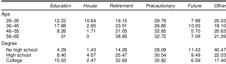
Figure 1 plots the means and the quartiles of net worth by age group for the two datasets (limited to the households also used in the estimation). Figure 2 does the same for net worth exclud-ing housexclud-ing wealth. Because of the concentration of wealth at the top of the distribution, the means are much higher than the medians and are usually closer to the third quartile. For college graduates in particular, means are more than twice as high as medians. The means in the SCF tend to be higher than those in the PSID, because by oversampling the rich, the SCF is able
Figure 1. Means (straight line), Medians (dashed line), and First and Third Quartiles (dotted lines) of the Distribution of Net Worth, by 5-Year Age Groups, 1992 Dollars.
Figure 2. Means (straight line), Medians (dashed line), and First and Third Quartiles (dotted lines) of the Distribution of Net Worth Excluding Main Housing, by 5-Year Age Groups, 1992 Dollars.
to give a better description of the top 5% of the distribution. However, as also shown in detail by Juster, Smith, and Stafford (1999), for lower quantiles the two datasets give similar infor-mation. The PSID is thus also a good dataset for this article, which focuses on the medians.
The estimation uses the following data. The SCF 1989, 1992, and 1995 waves are used, deating the values to 1992 dol-lars using the consumer price index (CPI) for urban consumers. Each observation is weighted according to the weight provided in each wave of the survey. For the PSID, all of the available waves (i.e., 1984, 1989, and 1994) are used. The census and the Latino sample are excluded, and equal weight is assigned to each observation in the remaining sample, which is repre-sentative of the whole population. Because the PSID is a panel, some households appear in more than one wave. Each house-hold is counted as a different observation each time it appears in a wave.
Only households age 26–65 (age and education refer to the age and education of the head) are used. Younger households are not included, because educational choice is not modeled. The older householdsare excluded because several features that are not modeled explicitly (e.g., the survival of one spouse, cer-tain types of medical shocks) may be relevant for their behavior. Only households composed at least by a head and a spouse are considered—singles were excluded (many singles are concen-trated among the very young and the old, which were already excluded). Singles include a large number of single mothers who are on welfare. Asset-based welfare programs can have relevant inuences on the savings decisions of the recipients (Hubbard et al. 1995) which are not fully captured in the present setup. Because these elements are not modeled, observations of singles are dropped. After also deleting the households with missing relevant demographic variables, the PSID sample in-cludes 1,039, 3,353, and 1,924 observations for households
without a high school degree, with a high school degree, and with a college degree, whereas the SCF sample includes 212, 1,100, and 1,963.
Two measures of wealth are considered. The rst measure, net worth, includes most assets [e.g., stocks, bonds, housing, and vehicles, as well as individual retirement accounts (IRAs) and thrift accounts] minus liabilities (e.g., mortgages, credit card debt). Pension wealth and capitalized social security are not part of net worth. In the model assets can be freely traded (or, equivalently, it is possible and costless to borrow against them at the constant rate of return R), and their payoff is the stream of interests that they give. Pensions and social secu-rity do not have these characteristics, because they are typi-cally nonfungible and usually provide a stream of earnings af-ter retirement. Therefore, they are accounted for in the earnings measure, as explained in Section 4.3. Many assets included in net worth are also not perfectly fungible; for instance, there are penalties in drawing money from IRAs, and markets that allow to borrow against them do not exist. However, because of the computational burden of accounting for these characteristics, IRAs and similar accounts are simply added to the other, more fungible forms of wealth. (Incidentally, note that the PSID, un-like the SCF, does not distinguish whether an asset is part of an IRA or of other more liquid forms.)
In particular, the inclusion of housing wealth may be prob-lematic. Housing wealth does, at least in part, constitute wealth for precautionary purposes. A house can be sold in case of particularly bad shocks, and ownership of a house per se pro-vides consumption insurance, because one does not have to pay rent, which is an important part of total consumption ex-penditures. However, selling a house can be expensive, and households rarely borrow against housing wealth for consump-tion purposes. Therefore, I also consider a second measure of wealth, net worth (as dened earlier) excluding primary hous-ing. Housing is assumed to enter the utility function separately from other forms of consumption, and it does not affect savings in other assets.
4.3 The Earnings Data
As explained in Section 3.2, the earnings process has three components: a common productivity growth factor,g; a senior-ity component,F.age;education); and a stochastic component,
u. The term g represents productivity growth in post-World War II United States. It is assumed to be constant over time and is common to all educational groups. Using aggregate data on workers’ compensation from the Bureau of Labor Statistics, it is calibrated togD:016.
The age–education earnings proles are estimated using data from the Consumer Expenditure Survey (CEX); see Appen-dix A for details on the exact equation. Two measures of earn-ings, corresponding to the two measures of wealth, are used.
As explained in the previous section, net worth does not in-clude pensions and social security wealth. Rather, pension and social security wealth is assumed to generate an income stream that is included in earnings. Savings in the form of pension and social security contributions is not part of the savings that in-creases the measure of net worth used, and thus these contribu-tions should not be counted in the earnings. The income mea-sure used is thus labor earnings, net of taxes, social security,
and pension contributions, and inclusive of pensions, social se-curity, and other transfer income (e.g., unemployment benets). Moreover, educational and medical expenditures are excluded, which can be considered committed expenditures that decrease income but do not give utility. CEX datasets are used rather than other datasets, such as the PSID, precisely because they contain detailed information about such expenditures.
The second set of estimates uses wealth net of primary hous-ing. For simplicity, it is assumed that housing wealth accumu-lates exogenously. Therefore, expenditures for housing, (i.e., mortgage down payments, interest payments, and housing addi-tions) are also excluded from the previous denition of income. For the stochastic component, the estimates of Carroll and Samwick (1997b), who used PSID data on before tax labor earnings, are used. Carroll and Samwick estimated a slightly different equation for u, which is, however, equivalent to the one used in this article. Appendix A explains the mapping. The resulting variances of the innovations´, ¾´2, equal .121, .090, and .070 for households with no high school degree, with high school, and college graduates, whereasà equals .59, .45, and .54. This implies that the variance of earnings decreases with education.
It should be noted that, although various types of transfer in-come (e.g., unemployment benets, Aid to families with De-pendent Children) are taken into account in constructing the mean income proles, minimum income levels or consumption oors are not explicitly modeled. As already pointed out in Sec-tion 4.2, when these features are explicitly introduced(as shown in Hubbard et al. 1995), the number of people with zero wealth increases. This may affect my results regarding the left tail of the wealth distribution, above all for lower education groups. However, only median wealth holdings are used in the present estimation. Moreover, only householdscomposed by a head and a spouse are used, whereas most of these programs are targeted to single-parent families.
Note also that some types of risks are also not explicitly in-cluded. Medical expenditures are excluded from the earnings proles, and their variability is not considered. They may be an important source of risk for the old (who are, however, not con-sidered in the estimation). The aggregate uncertainty coming from the business cycle is also not present, although typically the variability of the aggregate shocks is much smaller than the idiosyncraticcomponent (see, e.g., Storesletten, Telmer, and Yaron 1999).
5. THE RESULTS
This section presents the estimates of¯and° (Sec. 5.1), and their implications for precautionary savings (Secs. 5.3 and 5.4).
5.1 Estimates of the Rate of Time Preference
and Risk Aversion
Tables 2 and 3 show the estimates of¯and°, obtained using the condition on the medians (10) and on the means (14). Ta-ble 2 uses net worth, whereas TaTa-ble 3 uses net worth excluding housing wealth. A 3% after-tax real interest rate and no volun-tary bequests (®D0) are assumed.
First, consider the column for the medians, for the estimates obtained using total net worth. The results for all groups imply
Table 2. Estimated¯and°
Median Mean
NOTE: Standard deviations are in parentheses, andÂ2 results (for the means) are in on the third rows.
a relatively high coefcient of risk aversion (greater than 3, ex-cept for the lowest educational group) and, for the groups with-out a college degree, a low rate of time preference—a cong-uration suggesting that precautionary savings are quantitatively very relevant, as shown in the following sections. The estimates obtained using the PSID and those using the SCF are relatively close—not surprisingly, because, as explained in Section 4.2, the two datasets imply similar median wealth proles. Note in-cidentally that the SCF has few observations for the group with-out a high school degree, and the estimates have large standard errors; thus it is better to examine those from the PSID only.
College graduates have a higher degree of patience,¯, than the other two groups, that in turn have similar¯. For college graduates,¯ is around .98, whereas for the others it drops to around .95–.93. The relation between education and patience has been already studied by, for instance, Lawrance (1991), who estimated the degree of patience from Euler equations on consumption and found that it increases with education. Note, however, that the risk-aversion coefcient is also decreasing with education,which suggests that not only different time pref-erence, but also different attitudes toward risk can explain dif-ferent saving behaviors across groups.
The estimates obtained excluding housing wealth (Table 3) present a similar picture, with some differences. Housing
Table 3. Estimated¯and°, Net Worth Excluding Housing
Median Mean
wealth tends to be a large fraction of households’ wealth, par-ticularly for the relatively less afuent. Correspondingly, even correcting the earnings as explained in the previous section, there is a large drop in the estimated degree of patience for the lowest two educational group, with¯dropping to values around .84–.86. The drop of around .01 in the discount factor for the college graduates is instead smaller. The coefcient of risk aver-sion remains high (greater than 3) for all groups, although there is now little difference in the value between groups.
Regarding the difference in preferences between groups, Hubbard et al. (1995) have argued that social programs with asset-based means testing (i.e., transfers to people who have very low wealth holdings) induce many households with low lifetime income (most of them with low education levels) to hold little or no wealth. As previously mentioned, most of the households who are most affected by these programs are ex-cluded, and then only the median households are considered, with no attempt to match the lower quantiles. These correc-tions thus help control for the effect discussed by Hubbard et al. (1995). However, at least in part, the lower degree of patience and the lower degree of risk aversion of the households with-out a high school degree may reect not only genuine differ-ences in preferdiffer-ences, but also the impact of these programs. Including them (along the lines of, e.g., Hubbard et al. 1995) could therefore be an important extension of the model. How-ever, such extension would come at a very great computational cost, because the model would not be homogeneousin earnings anymore. Hubbard et al. (1995), moreover, showed that such programs have almost no impact on the median wealth holding of the college graduates. Therefore, the estimates for this group should not be affected.
5.2 Matching Means
Consider now the estimates obtained using the mean condi-tion (the right most columns in Tables 2 and 3). They imply either a much higher coefcient of risk aversion or a higher de-gree of patience (or both), above all for of college graduates.
The reason for this is that the means are affected by the right tail of the distribution of wealth, whereas the medians are not. Because of the high concentration of wealth, the richest house-holds hold a disproportionate share of total wealth. However, the model presented in this article is not able to adequately cap-ture the behavior of the very rich, because it does not consider the earnings levels and above all the large bequests received by the very rich. To match the observed mean wealth, the es-timates simply assign high patience and high risk aversion to all households. The effect is strong, particularly for the college graduates, because the richest households tend to be among this group.
For this reason, the estimates based on the means are biased upward and are inappropriate for the purpose of drawing infer-ence about most of the population. Incidentally, this exercise suggests that the parameters of the utility function used to cal-ibrate macroeconomic models of aggregate capital may differ from those found from microeconomic estimates. The behavior of the very rich has a large impact on the aggregates, and this group may be characterized by preferences and face different sources of risks than the rest of the population, on which many microeconomic estimates (including this one) are based. Thus the following sections concentrate on the rst set of estimates, those based on median wealth.
5.3 Precautionary Savings
The parameter estimates presented earlier imply that buffer stock wealth is a large component of the total wealth of the median household. It is difcult to exactly measure the contri-bution of precautionary savings to total wealth, because wealth accumulated for precautionary purposes is then available also for retirement. To get a rough idea, the following experiment is performed. For a given set of preference parameters, one can compute the wealth prole when there is earnings uncertainty (as done until now) and when earnings are certain. The latter is calledprole life cycle wealth. The difference between the sim-ulated wealth proles with and without earnings uncertainty can be considered the contribution of precautionary savings to total wealth.
In particular, three wealth proles are computed: the one pre-dicted by the precautionary saving model, the one prepre-dicted by the same model without earnings uncertainty and with borrow-ing constraints (so that households must hold a nonnegative amount of wealth), and the one predicted by the model with-out uncertainty and with the possibility of borrowing, so that households can borrow in certain periods and repay later. (This case can be considered the case of complete markets for the earnings uncertainty.) Note incidentally that longevity risk (i.e., about the age of death) is still present in all of the simulations. Only earnings are deterministic.
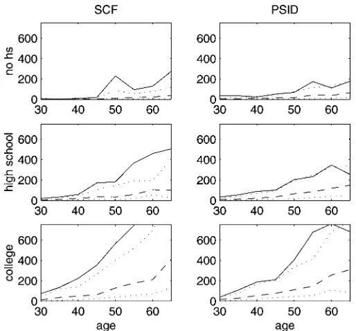
The implied wealth paths (for college graduates,®D0) are depicted in Figure 3. Figure 3(b) and (d) shows the empiri-cal paths.C/and the wealth paths computed from the model (dashed lines), with and without uncertainty. The top line is the precautionary saving model, whose parameters have been es-timated to match the data. When the precautionary motive is absent, households save much less. The estimates suggest that
(a) (b)
(c) (d)
Figure 3. Simulated Wealth Paths, With and Without Uncertainty, for (a) Net Worth and (c) Liquid Wealth, and Proportion of Wealth Attribut-able to Precautionary Savings, for (b) Net Worth and (d) Liquid Wealth, College Graduates.
(a) (b)
(c) (d)
Figure 4. Simulated Wealth Paths, With and Without Uncertainty for (a) Net Worth and (c) Liquid Wealth, and Proportion of Wealth Attribut-able to Precautionary Savings for (b) Net Worth and (d) Liquid Wealth, High School Graduates.
without the precautionary motive persons will not save early in life, because they expect higher income in the future. If they can borrow, they will do so until around age 40 (bottom line), and they will repay their debt later. If they cannot borrow (middle line), then they will keep little or no wealth early in life. Even-tually, households start saving for retirement, and the wealth prole becomes positive and rises until retirement at age 65. But the switch to retirement saving happens late, around age 45–50. These estimates thus conrm Carroll’s (1997)
sugges-(a) (b)
(c) (d)
Figure 5. Simulated Wealth Paths, With and Without Uncertainty, for (a) Net Worth and (c) Liquid Wealth and Proportion of Wealth Attribut-able to Precautionary Savings for (b) Net Worth and (d) Liquid Wealth, No High School Degree.
Figure 6. Value of the Objective Function (10), College Graduates, PSID. The minimum is .989 and 4.26.
tion about the relative importance of the motives for saving at different ages.
Precautionary wealth is thus an important component of total wealth. To stress this point even more, Figure 3(a) and (c) shows the fraction of total wealth attributable to precautionarysavings. This is computed as total wealth minus life cycle wealth over to-tal wealth (with the ratio set to 1 when toto-tal wealth is negative). The ratio is close to 1 until age 45–50, meaning that most of the wealth can be attributed to the precautionary motive. The ratio then decreases as households approach retirement, but it still remains high. Even at retirement, the level of wealth implied by the model with precautionary savings is twice as high as the level implied by the model without uncertainty. The results for high school graduates (Fig. 4) and for households without a high school degree (Fig. 5) are even starker, since these two groups are even more impatient than the college graduates.
5.4 Patience Versus Risk Aversion
Figure 6 shows the value of the objective function (10) for the case of college graduates in the PSID. The plot is relatively at along one direction; if° is xed and only¯ is estimated, then¯decreases as we increase°. The results of this exercise are reported in Table 4.
When risk aversion is increased, households accumulate more assets for precautionary purposes. Therefore, to match the
Table 4. Estimated¯, PSID (1984–1994), Using the Condition on the Medians (10), for Various°(Columns)
Net worth Excluding housing
1 6 1 6
College
1:009 :950 :998 :917 (:0004) (:003) (:0005) (:0038) High school
:996 :820 :991 :750
(:0003) (:0035) (:0002) (:0034) No high school
:988 :771 :982 :680
(:0005) (:0066) (:0009) (:009)
NOTE: Standard deviations are in parentheses.
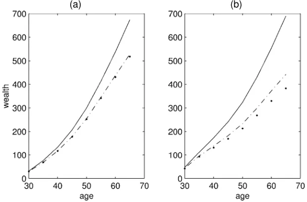
(a) (b)
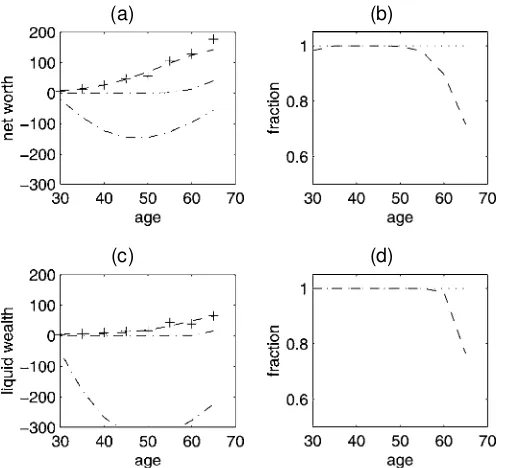
Figure 7. Wealth Paths, Net Worth (a) and Net Worth Excluding Pri-mary Housing (b), for College Graduates. Data (C),°D1 (dashed and dotted line) and°D6 (dotted line) and¯as in Table 4, Estimated¯and
°(dashed line).
same median amount of wealth requires decreasing¯ and as-suming less patience. The opposite occurs when° is decreased. However, the life cycle proles are different for different com-binations of the two parameters.
Figure 7 plots the implied wealth paths for° D1;6 and the corresponding estimates of ¯ shown in Table 4, and for the jointly estimated ¯ and ° from Section 5.1 (that imply a ° around 4). The estimates are from the PSID.
The proles for° around 4 (the estimated value), and° D6 are very close, which suggests that it may be difcult to iden-tify the two parameters for such values of °. The prole for ° D1 is, however, somewhat different from the other two; it implies relatively large savings very early in life, when agents save for the anticipated expenditures (described in Sec. 3.1) oc-curring around age 40, and when they quickly build up their buffer stock of wealth. The prole is rather at from 35 to 50, when consumption for demographic purposes (represented by the discount factor corrections) is highest. Less risk-averse households will save very little, or dissave, during this period, whereas more risk-averse ones will tend to save more to keep a higher buffer stock of wealth. Finally, after age 50, there is again accumulation of wealth for retirement purposes. When
° is higher, the required buffer stock of saving is higher, and there is more wealth accumulation also at later ages and during periods of high consumption needs (such as around age 40).
5.5 Consumption Proles
One of the reasons for the development of models with pre-cautionary savings was the observation that the prole of con-sumption over the life cycle is hump-shaped and tends to track that of income, a feature not replicated by the at proles of certainty equivalent models. Figure 8 plots empirical and simu-lated median proles for consumption and income for all three groups; the graphs refer to the experiment with housing wealth. The (smoothed) empirical consumption proles are obtained from the CEX (excluding the same type of households as for wealth and earnings).
The simulated proles tend to reproduce some aspects of the behavior of the empirical series. The consumption paths are very steep at the beginning of the life cycle, as is the income prole. Consumption then falls signicantly below income, as the household saves for retirement. And it exhibits the hump shape (except for college graduates, whose degree of patience is high—.989—and whose consumption peaks at retirement).
Relative to the data, the simulated proles tend to show a lit-tle more savings early in life (until age 35) for college graduates and high school graduates, but the opposite for people without a high school degree, who have the lowest risk aversion and time preference. This is due to the high estimates of risk aversion; young households are saving for precautionary motives, even if income will be much higher later in life.
This may explain the difference between the estimates of the present study and those of Gourinchas and Parker (2002), who looked at consumption proles and found lower estimates of the coefcient of risk aversion (between .5 and 1.5, depending on the group). The consumption paths that these authors generated imply consumption higher than income for householdsyounger than 30–35 years, which is consistent with consumption data. Wealth data instead tend to show much higher savings at that age, which the model explains as precautionary savings.
6. FURTHER IMPLICATIONS OF THE ESTIMATES
The previous section discussed the implications of the esti-mates of¯and° on the magnitude of the precautionary motive
(a) (b) (c)
Figure 8. Median Consumption Simulated (solid line) and Data (dashed line), and Income (dotted line) Paths for the Three Educational Groups: (a) No High School, (b) High School; (c) College.
for saving. In this section some further implications are exam-ined, to highlight the fact that a careful choice of these parame-ter is also important for other economic questions.
Simulations of life cycle models are often used to study how households increase their savings in response to various taxes and incentive schemes. For instance, Summers (1981) showed that in a life cycle model without uncertainty, savings are very interest-elastic, and thus small changes in taxes on capital can generate large increases in capital accumulation. This may not be true in a precautionary savings model, however. If precau-tionary motives are important, then people want to accumulate a buffer stock of wealth, but changes in interest rates do not in-crease their savings much beyond that point. Savings are thus very interest-inelastic. As shown by Cagetti (2001), the value of the elasticity depends on the combination of¯and° chosen to simulate the model.
This point has been made by others, including Carroll (1997), and is the basis for the results of Engen et al. (1996) on the im-pact of saving incentive schemes. There is a large literature ex-amining the effects of IRAs. Some authors (e.g., Poterba, Venti, and Wise 1996) found large effects. However, a model with pa-rameter values similar to those of the present study (such as that of Engen et al. 1996) implies very small effects. The results in this paper thus conrm the choice of their parametrizations.
Of course, even if the median household is very interest in-elastic, a considerable proportion of total capital is concentrated in a small fraction of the population, who may have different savings behavior. Therefore, capital accumulation may be very interest-elastic in the aggregate, if this small fraction of house-holds is responsive to changes in interest rates.
6.1 Heterogeneity in the Discount Factor
Heterogeneityin the degree of patience is often considered an important factor in explaining the dispersion of wealth. For in-stance, Krusell and Smith (1998) reproduced the variability of wealth holding (in an innitely lived agent model) by assum-ing two types of agents, who have slightly different discount
factors. In the absence of precautionary savings, savings are ex-tremely sensitive to the choice of¯. In the standard, innitely lived agent model with quadratic utility (the certainty equiva-lence model), one must assume that¯RD1. If individualswere more patient, they would accumulate wealth without bounds.
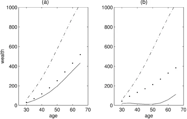
But, when precautionary savings are important, larger dif-ferences in patience are needed to generate large dispersion in wealth. Figure 9 shows how the median wealth (net worth) pro-le changes when the discount factor is changed while keep-ing ° xed. Figure 9(a) is for the estimated ° D4:26, and ¯D:969; :989, and 1.09. Figure 9(b) shows a similar experi-ment, but when precautionary savings are less important (° D 1,¯D:98;1:00;1:02). When° D1, changes in the discount factor have a large impact on the amount of wealth held at re-tirement, but the impact is lower when° D4:26, above all when moving¯away from 1.
The present estimates, however, do suggest also large differ-ences in the rate of time preference among groups, sometimes greater than .05. Carroll (2000a) showed that with precaution-ary savings and differences in¯ of the magnitude of those be-tween my estimates for different educational groups, one can generate signicant dispersion in wealth holdings (and interest-ing macroeconomic dynamics not captured by the representa-tive agent model). This article points out, however, that differ-ences in risk aversion can be equally important in explaining differences in behavior across households.
6.2 Bequest Motives
It has been assumed until now that there are no bequest mo-tives (®D0). When® >0, households have an additional mo-tive for saving, and, for a given level of¯ and°, they will ac-cumulate more wealth. This section examines how the wealth prole change with® >0.
Here® is calibrated to two other values, chosen so that the marginal propensity to consume in the last period is .5 and .1. That is, a person who is sure to die would leave 50% and 90% of his own wealth to the children (®D0 obviously implies a
(a) (b)
Figure 9. Wealth Paths (net worth), for°D4:26 (a) and°D1 (b) for College Graduates. Low¯(solid line), medium¯(dotted line) and high¯
(dashed and dotted line).
(a) (b)
Figure 10. Wealth Paths (net worth) for°D4:26 (a) and°D1 (b), Various®, for College Graduates.
marginal propensity to consume of 1, because the person would consume everything and leave no bequests). Figure 10 shows the wealth proles before retirement for the three choices of ®, (a) for the estimated¯ D:989 and ° D4:26, and (b) for ° D1 and the corresponding¯ D1:00. Note that the actual parameters®chosen are different in the two panels, because the marginal propensity to consume in the last period also depends on¯ and°. The actual parameter values are 1 and 10,000 for 10(a) and 1.07 and 7.7 for 10(b).
For the estimated parameter values, there is almost no dif-ference in switching to a marginal propensity to consume of .5, whereas the wealth path for the case of a propensity of .1 is 15% higher at retirement. This suggests that®has a relatively small effect on wealth proles before retirement, unless a very high degree of altruism is assumed. For the other parameter cong-uration (low risk aversion and high patience), the differences in the wealth path are a somewhat higher (for instance, the wealth at retirement increases by 50% when the altruism parameter is at its highest value). The reason for the difference is that the utility from bequest is obtained only at the time of death and thus is more heavily discounted by more impatient households, such as the ones in Figure 10(a). Bequest motives, therefore, do not much affect the behavior of impatient households, but matter more for more patient ones.
These results show that it is difcult to identify bequest mo-tives from (median) wealth data before retirement; thus in most of the article® is set to 0. To identify the presence of bequest motives, it may be necessary to look at data on the very old (that has been excluded from this analysis), and on whether, and if so, how they run down their wealth. Moreover, the be-quest motive can be quantitatively important in explaining the wealth holding of a subgroup of (very rich) households, as il-lustrated by De Nardi (2000), who showed that bequest motives can account for part of the wealth concentration in the hands of the top 1% of the population. It is also important to note that the results depend on the particular way of introducing bequest motives. These motives may enter the utility function in a dif-ferent way—in particular, providing utility not only at the time of death, but also during the lifetime.
7. CONCLUSIONS
This article has assessed the importance of precautionary savings for the accumulation of wealth by formally estimating a life cycle model of consumption and saving. Age proles of wealth holdings were constructed and the preference parame-ters (time preference and risk aversion parameparame-ters) found that generate simulated proles closest to those constructed from microeconomic data (PSID and SCF). The observed life cycle proles are consistent with a low degree of patience, a high degree of risk aversion, and differences in the degree of pa-tience among various educational groups. Under such a con-guration, saving is dictated by precautionary motives early in life, and concerns for retirement are important only for older households. Precautionary motives explain a large fraction of the wealth of the median household. The amount of wealth at retirement implied by the model with precautionary savings is twice as high as that implied by a pure life cycle model without uncertainty.
The model and the estimation methods presented in this ar-ticle can be applied to more complex settings. First, various models of wealth accumulation have been simulated to exam-ine portfolio composition over the life cycle (e.g., Campbell and Viceira 2002), or the effects of different social security and pen-sion schemes (e.g., Samwick 1998). The results of these experi-ments depend on the extent of precautionary savings; it is there-fore fundamental to choose appropriate preference parameters used to perform such exercises. Second, most models, includ-ing this one, fail to account properly for the extreme concen-tration of wealth among the richest households. A richer setup, involving a better characterization of the income and returns to entrepreneurial activities, may be helpful in analyzing such phe-nomenon. Finally, the analysis presented here suggests that bor-rowing constraints, preference heterogeneity, and life cycle be-havior can interact in ways not captured by the simplied, in-nitely lived representative agent models common in the macro-economic literature. Some contributions on the importance of heterogeneity and market incompleteness for general equilib-rium have begun to appear (Browning, Hansen, and Heckman 1999; Carroll 2000a), but the problem deserves further study.
ACKNOWLEDGMENTS
The computer codes and the data are available on request or at http://www.people.virginia.edu/˜ mc6se/. I received sugges-tions from seminar participants at many institusugges-tions. I would like to thank in particular Francisco Ciocchini, Mariacristina De Nardi, Eric French, James Heckman, Manuel Lobato, An-namaria Lusardi, Jonathan Parker, Annette Vissing-Jørgensen, my advisor Lars Peter Hansen, the associate editor, and two anonymous referees. Financial support from the Margaret Reid Fund is gratefully acknowledged.
APPENDIX A: THE EARNINGS PROCESS
Figure A.1 displays the deterministic component of earnings. The dotted line represents college graduates; the straight line, households with a high school degree; and the dashed line, for those without. As mentioned in the text, the productivitygrowth factor is calibrated from total workers’ compensation data. The age and education component is estimated from a regression of CEX data about log earnings on a fourth-degree polynomial in age (separately for each educational group). The two pan-els correspond to the two measures of earnings described later. The drop at age 65 is generated by the assumption that house-holds retire after that age. The regression is estimated separately for working and retired household. A household is dened as retired if the head works for less than 500 hours and is older than 60.
Income and expenditure data from the Consumer Expen-diture Survey, in the extracts prepared by Sabelhaus, avail-able on the National Bureau of Economic Research website at
http://www.nber.org/ces_cbo.htmlare used. As explained in the main text, because marital risk is not considered, only house-holds with a head and a spouse are considered. For retired peo-ple, however, all households are considered, to capture the fact that one of the spouses may die, but savings decisions may be made considering the welfare of the survivor. Observations with
missing demographic information, those with an incomplete re-port for any quarter, and those with income of less than $500 1992 dollars are excluded. Apart from very few cases of busi-ness or nancial losses, zero earnings most likely represent in-accurate data, given the inclusion of various transfer income in the measure of earnings.
Two denitions of earnings are used, depending on the ex-periment. For the experiment with net worth, earnings represent all sources of nonasset income, net of taxes. The CEX reports federal, state, and social security taxes paid by the household. The ratio¸of labor income over total income (setting asset in-come to 0 if it is negative) is computed, and such fraction of the taxes is assigned to labor income. Then property taxes, pen-sion contributions, medical, and educational expenditures, are subtracted from this measure.
Health expendituresshould be considered a negative shock to income. For instance, Hubbard et al. (1995) explicitly modeled a random process for medical expenditures, which adds another dimension of variability to the stream of income. For simplic-ity, medical expenditures are subtracted when constructing the average proles for income, but the randomness of such expen-ditures is not considered explicitly. Such randomness can be an important reason for precautionary savings, above all for the old. Educational expenditures are excluded because they are to some extent precommitted, and there is an important life cycle component in their timing; that is, they cannot be smoothed. Agents save at the beginning of the life cycle to nance these expenditures. Therefore, they are subtracted from income and considered an (anticipated) negative shock to earnings.
The second denition of earnings, that used when looking at net worth excluding primary housing, subtracts from the in-come measure explained above also all expenditures related to the accumulation of housing wealth, that is, mortgage pay-ments, housing additions, and rents. Other expenditures on housing, such as heating and cleaning, are not excluded, be-cause such expenditures can be considered current consump-tion. Note that mortgage down payments are also subtracted from income. Because of this, there are some households for
(a) (b)
Figure A.1. Estimated Earnings Proles for the Three Educational Groups, in Thousands 1992 Dollars, CEX 1980–1995. (a) Prole used in the estimation with net worth. (b) Prole used in the estimation with net worth excluding housing.
whom the implied measure of earnings is below $500 or nega-tive (approximately 6% of the sample). Because logarithms are taken, such observations are excluded.
For the stochastic component of earnings 7, the results of Carroll and Samwick (1997) are used. They estimate a slightly different process,
utDut¡1C O´tC O²t¡ O²t¡1:
Basically, the innovationin the present formulation is an MA(1) process, whereas Carroll and Samwick (1997) gave it a perma-nent (´Ot) and a purely transitory component (²Ot). The two for-mulations are observationally equivalent, in the sense that they generate the same autocovariances for ut. If a process with a certain¾´ andà (the parameters that characterize the MA(1) formulation) is assumed, then an equivalent process of the form assumed by Carroll and Samwick (1997), that is, a process that for a certain¾²O and¾´O generates the same variances and auto-covariances, can be found. Given the estimates of¾²O and¾´Oof Carroll and Samwick (1997),¾´ andà thus can be recovered. To do so, the variance and the rst-order autocorrelation of1ut (a system of two equations in the two unknowns¾´andÃ) are equated.
To simulate the model, I need to initialize the cross-sectional distribution of earnings at age 25 must be initialized. For sim-plicity, this distribution is assumed to be lognormal, with a mean and a variance equal to the empirical ones; a grid of initial income levels (5 in the present simulation) is then cho-sen using Gauss–Hermite gridpoints and weights. For instance, for college graduates, this implies a weight of .53 at the mean of $30,000, with the highest initial point being $95,000, with weight .01. Given the initial level of income, the initial wealth-to-income ratio is then initialized at its observed distribution. Three initial values are chosen, corresponding to the quantiles .17, .5, and .83 of the wealth-to-income ratio.
APPENDIX B: BEQUESTS AND DEMOGRAPHIC CORRECTIONS
Figure B.1 plots the probability that a household receives a bequest as a function of age. The data is taken from reported
gifts and bequests in the PSID. This probability is modeled with a probit,
Pr.bequest/D8.®e¤educCP.t//;
where8is the normal cumulative distribution function,educ
is a dummy variable for education, andP.t/ is a third-degree polynomial in age. This formulation implies that the life cycle proles of the probabilities for different educational groups dif-fer only by a multiplicative constant. An attempt was made to estimate education-specic age coefcients, but the estimates were very imprecise.
The median bequest-to-income ratio (conditional on receiv-ing a bequest) was also estimated, and it was assumed that when receiving an inheritance, the household receives this propor-tion of his income. This ratio does not seem to depend signi-cantly on age, so it is considered a constant. The ratios for the three educational groups are 1.16, 1.07, and .96. Note that the PSID does not capture the bequests left by very rich households, which, as noted by, for instance, Kotlikoff and Summers (1981), constitute a signicant fraction of the total wealth in the econ-omy. These bequests are fundamental in explaining the concen-tration of wealth in the right tail of the distribution, as shown by De Nardi’s (2000) model of wealth accumulation with intergen-erational linkages. However, this article focuses on the median wealth holding.
As suggested by Attanasio et al. (1999), the discount factor ¯ is corrected to capture the effect of demographic variables on consumption. The correction has the exponential form,eZtµ.
Zincludes log family size and log hours of leisure of the spouse (computed as 5,000 minus the number of hours worked in the year). The estimate forµ is taken from Attanasio et al. (1999). The average prole of the two demographic variables over the life cycle,bZt, is computed and then the implied corrections, ebZtµ, shown in Figure B.2, are calculated. For simplicity, this
discount factor is assigned to all households in the simulations instead of using different demographic proles for each house-hold. Thus there is no uncertainty coming from the discount factor.
Figure B.1. Estimated Probability of Receiving a Bequest, PSID 1969–1989 ( college;¢–¢– high school;¢ ¢ ¢ ¢ no high school).
Figure B.2. Discount Factor Corrections (: : :no high school;¡ ¡ ¡
high school;¢ ¡ ¢¡college).
Note that the shape differs between education groups only because the prole of the demographic variables is different (due mainly to the fact that college graduates have children later). There is no education dummy inµ.
APPENDIX C: THE ESTIMATION METHOD
To exploit the median restriction (10), the method described by Powell (1994) is used. Powell (1991) gave conditions for consistency and asymptotic normality.
Let» D[¯; °]0be the set of preference parameters to be
esti-mated. For each age groupt(in this case, for each of the 5-year age groups), the¼th quantile can be dened as
E.¼¡1.wti·mt.» //jt/D0; (C.1)
wherewti is the wealth of an individualibelonging to groupt,
mtis the¼th quantile of the distribution of wealth for each age group, and 1is the indicator function.mt also solves the loss function
and the true parameter»0solves
min
The previous restrictions are conditionalon the age groupt. The unconditionalcounterpart,
min » E.½¼.w
t
i¡mt.» //q.t//; (C.5)
where q.t/ is some weighting function, can be formed. The sample analog is observations, and!iis the weight of observationiin the entire population.
Because no analytic expression exists form,mmust be ulated; then the cumulative distribution function between sim-ulated points is linearly interpreted. The variance of the esti-mator due to the simulation is not considered; however, the life cycle proles are simulated for 10,000 households while each age group contains from 20 to 100 observations, so the ratio of observations to simulated points is extremely low.
An efcient choice ofq.t/isf.mtjt/, that is, the density of the distribution of wealth of agents of agetat the median. With this choice, the estimator»O has a distribution
p
and this value is used in a second round of estimation.Of is a nonparametric estimate with Gaussian kernel.
Experiments using means (condition 13) instead of medians were also performed, using a simulated method-of-momentses-timator. Letwi be the observed wealth of individuali.Wt.» / is the (theoretical) mean wealth of individuals of aget for the parameter value», andWst.» /is the simulated average wealth level of individuals of the age group t, again for parameter value». The moment conditions (one for each age groupt) are
E¡1.t/.wi¡Wt/
¢
D0; (C.9)
where1./is the indicator function, which has value 1 ifti, the age of individuali, equalstand 0 otherwise. The expected value is not conditional on age (i.e., it is taken over all households).
Observations taken from the datasets are weighted differently (see Sec. 4.2); therefore, one must construct the empirical coun-terpart to the foregoing moments using weights. LetwOti
i be the wealth observation on a household that has agetiand a weight !i in the total sample (the weights are here normalized to 1). The empirical counterparts to the foregoing moments are
b
In the rst stage, the identity weighting matrix is used to min-imize
b
M0IMb (C.11)
with respect to». Using the computed»O, an estimatebÄof the covariance matrix can be constructed,
ÄDvar¡1.t/.wi¡Wst/
¢
: (C.12)
The off-diagonal elements are 0. The elements on the diagonal are estimated by
X
i
!i.wti¡Wst/2: (C.13)
TDÄ¡1is the optimal weighting matrix, so in the second stage b
M0Äb¡1Mb (C.14)