56
1. The Result of Pre Test of Experiment Group
In this section, it was described the data obtained of pre test of
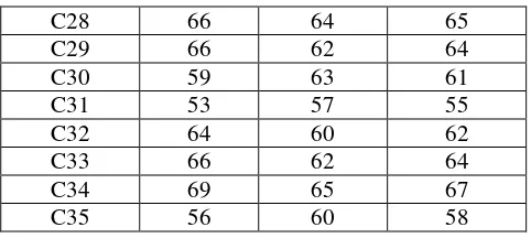
experiment group. The pre test was taken on Saturday, 3rd May 2014 at 12.00 – 13.30 in class X-7. They were 35 students who followed this test. The pre test scores of the experiment group were presented in table 4.1.
Table 4.1
C28 66 64 65
The distribution of students’ pre test scores of experiment group can also be seen in the following figure.
Figure 4.1 Histogram of Frequency Distribution of Pre Test Scores of Experiment Group
The figure 4.1 showed the pre test scores of students of experiment
group. It can be seen that there was a student got score 55, 59, 63, 69, 70,
and 71. There were two students got score 57, 60, 61, 62, 66, and 68.
There were three students got score 58 and 67. There were five students
got score 64. And there were six students got score 65.
0
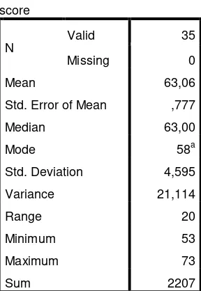
Table 4.2
The Table of Calculation of Mean, Standard Deviation, and Standard Error of Mean of Pre Test Scores in Experiment Group Using SPSS 21 Programs
Statistics
2. The Result of Pre Test of Control Group
In this section, it was described the data obtained of pre test of
control group. The pre test was taken on Thursday, 24th April 2014 at 10.00 – 11.30 in class X-1. They were 35 students who followed this test. The pre test scores of the control group were presented in table 4.3.
Table 4.3
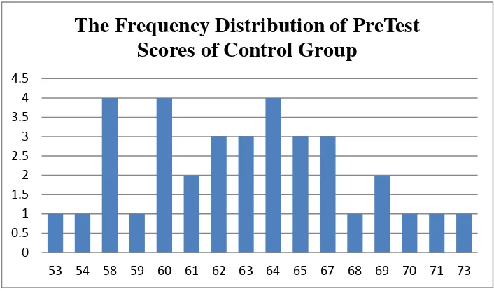
Figure 4.2 Histogram of Frequency Distribution of Pre Test Scores of Control
Group
The figure 4.2 showed the pre test scores of students of control
group. It can be seen that there was a student got score 53, 54, 59, 68, 70,
71 and 63. There were two students got score 61 and 79. There were three
students got score 62, 63, 65, and 67. There were four students got score
58, 60, and 64.
0 0.5 1 1.5 2 2.5 3 3.5 4 4.5
53 54 58 59 60 61 62 63 64 65 67 68 69 70 71 73
Table 4.4
The Table of Calculation of Mean, Standard Deviation, and Standard Error of Mean of Pre Test Scores in Control Group Using SPSS 21 Program
Statistics
3. The Result of Post Test of Control Group
In this section, it was described the obtained data of improvement
the students’ writing scores after taught without using Mind Mapping technique. The post test was taken on Saturday, 31st May 2014 at 10.00 – 11.30 in class X-1. They were 35 students who followed this test. The
post test scores of the control group were presented in table 4.5.
Table 4.5
C07 72 70 71
The distribution of students’ post test scores can also be seen in the following figure.
Figure 4.3 Histogram of Frequency Distribution of Post Test Scores of Control Group
The figure 4.3 showed the post test scores of students of
control group. It can be seen that there was a student got score 79, 76,
74, 69, and 64. There were three students got score 67 and 73. There
were four students got score 72, 68, and 66. There were five students
got score 70. And there were seven students got score 71.
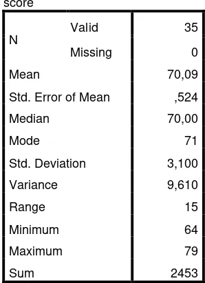
Table 4.6
The Table of Calculation of Mean, Standard Deviation, and Standard Error of Mean of Post Test Scores in Control Group Using SPSS 21
Programs
Statistics score
N Valid 35 Missing 0
Mean 70,09
Std. Error of Mean ,524 Median 70,00
Mode 71
Std. Deviation 3,100 Variance 9,610
Range 15
Minimum 64
Maximum 79
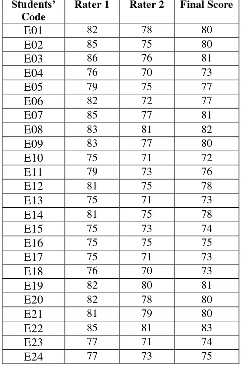
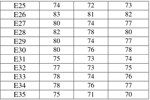
4. The Result of Post Test of Experimental Group
In this section, it was described the obtained data of improvement
the students’ writing scores after taught using Mind Mapping technique.
The post test was taken at Saturday, 31st May 2014 at 12.00 – 13.30 in class X-7. They were 35 students who followed this test. The post test
scores of the experimental group were presented in table 4.7.
Table 4.7
E25 74 72 73
The distribution of students’ post test scores can also be seen in
the following figure
Figure 4.4 Histogram of Frequency Distribution of Post Test Scores of Control Group
The figure 4.4 showed the post test scores of students of
experiment group. It can be seen that there was a student got score 83,
72 and 70. There were two students got score 82 and 76. There were
three students got score 81, 78, 75, and 74. There were five students
got score 77. There were six students got score 80. And there were
seven students got score.
Table 4.8
The Table of Calculation of Mean, Standard Deviation, and Standard Error of Mean of Post Test Scores in Experiment Group Using SPSS 21
Programs
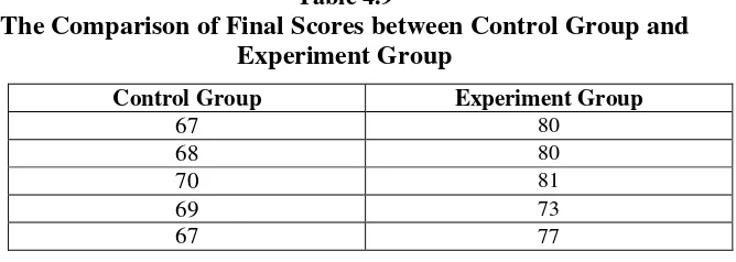
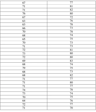
Based on the data above, it can be seen the comparison in Table 4.9.
Table 4.9
The Comparison of Final Scores between Control Group and Experiment Group
Control Group Experiment Group
67 80
68 80
70 81
69 73
67 77
6. Testing of Normality and Homogeneity
a. Testing of Normality
One of the requirements in experimental design was the test of
normality assumption. Because of that, the writer used SPSS 21 to
measure the normality of the data. Test Normality of Pre Test and Post
Test Scores were described in Table 4.11.
Description:
If respondent > 50 used Kolmogorov-Sminornov
If respondent < 50 used Saphiro-Wilk
The criteria of the normality test Pre Test and Post Test is if the
value of r (probability value/critical value) is higher than or equal to
the level of significance alpha defined (r ≥ α = 0.05), it means that, the
Variance 11,353 9,610
Range 13 15
Minimum 70 64
Maximum 83 79
Sum 2695 2453
Table 4.11
Tests of Normality
distribution is normal. Based on the calculation using SPSS 21 above,
the value of r (probably value/critical value) from Pre test and Post test
of the control group and experimental group in
Kolmogorov-Sminornova was higher than level of significance alpha used or r = 0.082> 0.05 (Pre Test) and r = 0.064> 0.05 (Post Test) so that the
distributions are normal. It meant that the students’ scores of in Pre
Test and PostTest had a normal distribution.
b. Testing of Homogeneity
The definition of Homogeneity of Variance is when all the
variables in statistical data have the same finite or limited variance.
When homogeneity of variance is equal for a statistical model, a
simpler computation approach to analyzing the data can be used due to
a low level of uncertainty in the data. Because of that, the writer used
SPSS 21 to measure the homogeneity of the data.
Table 4.12
Test of Homogeneity of Variance Levene Statistic
df1 df2 Sig.
score
Based on Mean ,120 1 68 ,730 Based on Median ,171 1 68 ,680 Based on Median and with
adjusted df
,171 1 65,457 ,680
From the table output above can be known that the value of
significance higher than 0.05 so can be concluded that the data have
the same variance or homogene.
B. Data Analysis
1. Testing Hypothesis Using ttest Manual Calculation
The writer chose the level of significance in 5%, it mean that
the level of significance of the refusal null hypothesis in 5%. The
writer decided the level of significance at 5% due to the hypothesis
type stated on non-directional (two-tailed test).It meant that the
hypothesis cannot directly the prediction of alternative hypothesis. To
test the hypothesis of the study, the writer used t-test statistical
calculation. First, the writer calculated the standard deviation and the
standard error of X1 and X2. It was found the standard deviation and
the standard error of PostTest of X1 and X2 at the previous data
presentation. It was described in Table 4.13.
Table 4.13
TheStandard Deviation and Standard Error of X1 and X2
Variable The Standard Deviation The Standard Error
X1 3,369 ,570
X2 3,100 ,524
Description:
The table showed the result of the standard deviation
calculation of X1 was 3.369 and the result of the standard error mean
calculation was 0.570. The result of the standard deviation calculation
of X2 was 3.100 and the result of the standard error calculation was
0.524.
The next step, the writer calculated the standard error of the
differences mean between X1 and X2 as follows:
Standard Error of the Difference Mean scores between Variable I and
Variable II:
SEM1- SEM2 = √
SEM1- SEM2 = √
SEM1- SEM2 = √
SEM1- SEM2 = √
SEM1- SEM2 = 0.77425835 = 0.774
The calculation above showed the standard error of the differences
mean between X1 and X2 was 0.774. Then, it was inserted theto
formula to get the value of tobserved as follows:
to =
to =
to =
With the criteria:
If ttest (tobserved) > ttable, Ha is accepted and Ho is rejected.
If ttest (tobserved) < ttable, Ha is rejected and Ho is accepted.
Then, the writer interpreted the result of ttest. Previously, the writer
accounted the degree of freedom (df) with the formula:
Df = (N1 + N2) - 2
stated on non-directional (two-tailed test). It meant that the hypothesis
cannot direct the prediction of alternative hypothesis.
The calculation above showed the result of ttest calculation as in the
Table 4.14.
Table 4.14 The Result of ttest
Variable tobserved
X1 = Experimental Group X2 = Control Group
tobserved = The Calculated Value
ttable = The Distribution of t value
Based on the result of hypothesis test calculation, it was found
that the value of tobserved was greater than the value of ttable at the level
of significance in 5% or 1% that was 2.000 < 8,934 >2.660 It meant
Ha was accepted and Ho was rejected.
It could be interpreted based on the result of calculation that
Ha stating that “the students taught by Mind Mapping technique gain better writing achievement” was accepted and Ho stating “the students
taught by Mind Mapping technique do not gain better writing
achievement” was rejected. It meant that teaching writing by using
Mind Mapping technique increases the 10th grade students’ writing scores at MAN Model Palangka Raya.
2. Testing Hypothesis Using SPSS 21 Program
The writer applied SPSS 21 program to calculated ttest in
testing hypothesis of the study. The result of the ttest using SPSS 21
program was described in Table bellow.
Table 4.15
Standard Deviation and Standard Error of X1 and X2 Group Statistics
Group Statistics
code N Mean Std. Deviation Std. Error Mean
score
Table 4.16
The Calculation ttest Using SPSS 21 Independent Samples Test
Independent Samples Test Levene's Test
for Equality of Variances
t-test for Equality of Means
F Sig. t df Sig.
(2-control group had difference scores of variance, it found that the result
of tobserved was 8,934.
To examine the truth or false of null hypothesis stating that
using Mind Mapping technique does not increase the 10th grade
students’ writing scores, the result of ttest was interpreted on the result
(df) was 68, it found from the total number of students in both group
minus 2.
Table 4.17
The Result of tobserved and ttable/ttest Variable tobserved
ttable
Df
5% 1%
X1-X2 8.934 2.000 2.660 68
The interpretation of the result of ttest using SPSS 21 Program,
it was found the tobserved was greater than the ttable at 1% and 5% the
level significance or 2.000 < 8.934 > 2.660. It could be interpreted
based on the result of calculation that Ha stating that “the students
taught by Mind Mapping technique gain better writing achievement” was accepted and Ho stating “the students taught by Mind Mapping technique do not gain better writing achievement” was rejected. It
meant that teaching writing by using Mind Mapping technique
increases the 10th grade students’ writing scores at MAN Model Palangka Raya.
C. Discussions
The result of the data analysis showed that the Mind Mapping
technique gave significance effect on the students’ writing scores for the 10th
graders of MAN Model Palangka Raya. The students who were taught using
without using Mind Mapping technique. It was proved by the mean scores of
the students who were taught using Mind Mapping technique was 77.00 and
the students who were taught without using Mind Mapping technique was
70.09. Based on the result of hypothesis test calculation, it was found that the
value of tobserved was greater than the value of ttable at 5% and at 1% the level of
significance or 2.000 < 8.934 > 2.660. It meant that Ha was accepted and Ho
was rejected.
In addition, the result of ttest calculation using SPSS 21 found that the
Mind Mapping technique also gave significance effect on the students’ writing scores. It proved by the value tobserved was greater than ttable both at 1%
and 5%the level of significance or 2.000 < 8.934 > 2.660.
Those statistical findings were suitable with the theories as mentioned
before that Mind Mapping can make the students easy in understanding the
material because it has a simple pattern that easy to remember. By using
picture and color, Mind Mapping can be funny to learn, it makes the brain
enjoy and excited in thinking something about the topic. Mind Mapping is one
of techniques in pre writing activity that allow the writer think more
creatively. The Mind Mapping was interested and makes students easy to
Mind Mapping is also one strategy that allows students to demonstrate
their understanding of the relationship among ideas within a text and to
visually present a hierarchy of ideas in a diagram format. Mind Mapping
helps people to think more effectively as a group without losing their
individuality. It helps groups to manage the complexity of their ideas without
trivializing them or losing detail.
There are reasons why using Mind Mapping technique gives effect on
the students’ writing ability of the 10th graders of MAN Model Palangka Raya. First, by using Mind Mapping, the students could memorize some new
words easily, by connecting their previous knowledge. Second, Mind
Mapping was an interesting technique for the students. It was shows from the
students’ response that they were very enthusiastic when they were taught by
using Mind Mapping. Third, the vocabulary in Mind Mapping was classified
into the specific categories. For example, in the topic of “Animal”, the
vocabulary was classified into some categories such as the colors, the
appearance, behaviors, habituates, etc. It makes the students easier to develop