CHAPTER IV
DATA FINDING AND DISCUSSION A. Data Finding
In this chapter, the writer presented the obtained data. The data were
presented in the following steps.
1. Distribution of the Experimental Group Scores
a. Distribution of Pre Test Scores of the Experimental Group
The pre test scores of the experimental group were presented in the
following table.
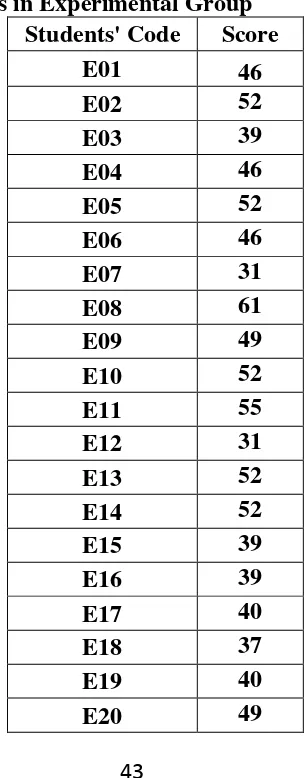
Table 4.1 The Description of Pre Test Scores of The Data Achieved by The Students in Experimental Group
Students' Code Score
E01 46
E02 52
E03 39
E04 46
E05 52
E06 46
E07 31
E08 61
E09 49
E10 52
E11 55
E12 31
E13 52
E14 52
E15 39
E16 39
E17 40
E18 37
E19 40
E20 49
E21 43
E22 31
E23 58
E24 55
E25 52
E26 34
E27 53
E28 51
Based on the data above, it was known the highest score was 61 and the
lowest score was 31. To determine the range of score, the class interval, and
interval of temporary, the writer calculated using formula as follows:
The Highest Score (H) = 61 The Lowest Score (L) = 31
The Range of Score (R) = H – L + 1 = 61 – 31 + 1 = 31
The Class Interval (K) = 1 + (3.3) x Log n = 1 + (3.3) x Log 28 = 1 + (3.3) x 1.447158031 = 1 + 4.775621502
= 5.775621502 = 6
Interval of Temporary (I) =
6 31
K R
= 5.1666666667 =5
So, the range of score was 31, the class interval was 6, and interval of
temporary was 6. Then, it was presented using frequency distribution in the
following table:
Table 4.2 The Frequency Distribution of the Pre Test Scores of the Experimental Group
Class (k)
Interval (I)
Frequency (F)
Midpoint (X)
The Limitation
of Each Group
Relative Frequency
(%)
Cumulative Frequency
3 46 – 50 5 47 45.5 – 51.5 17,85 57,14 4 41 – 45 1 42 40.5 – 46.5 3,57 39,28 5 36 – 40 6 37 35.5 – 41.5 21,42 35,71 6 31 – 35 4 32,5 30.5 – 36.5 14,28 14,28
∑F = 28 ∑P = 100
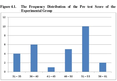
Figure 4.1. The Frequency Distribution of the Pre test Score of the Experimental Group
The table and figure above shows the pre test score of students in
experiment group. It could be seen that there were 4 students who got score 31 –
35. There ware 6 students who got score 36 – 40. There was a student who got
score 41 – 45. There were 5 students who got 46 – 50. There ware 10 students
who got 51 – 55 and there were 2 students who got 56 – 61. In this case, so many
students got point 51-55 and just a student got point 41-45 in the pretest. The
conclusion is vocabulary of student less and should have new media to increase
the vocabulary.
The next step, the writer tabulated the scores into the table for the
calculation of mean, median, and modus as follows:
0 2 4 6 8 10 12
Table 4.3 The Calculation of Mean, Median, and Modus of the Pre Test Scores of the Experimental Group
(I) (F) (X) FX fk (b) fk (a)
56 – 61 2 58 116 28 2
51 – 55 10 52 520 26 12
46 – 50 5 47 235 16 17
41 – 45 1 42 42 11 18
36 – 40 6 37 222 10 24
31 – 35 4 32,5 130 4 28
∑F = 28 ∑FX= 1265
a. Mean
Mx = ∑𝑓𝑋
𝑁 = 28 1265 = 45,178571429 = 45,17
b. Median Mdn = ℓ +
1 2𝑁−𝑓𝑘𝑏
𝑓𝑖 𝑥𝑖 = 5 2 11 14 5 .
46
= 5
2 3 5 .
46
=
46
,
5
7
,
5
=
54
c. ModusMo = ℓ + 𝑓𝑎
𝑓𝑎+𝑓𝑏 𝑥𝑖
= 5
1 10
10 5
.
46
= 5
11 10 5 .
46
=
46
.
5
4
.
5454
=51
,
04545
=
51
.
045
The calculation above shows of mean value was 45,17, median value was 54
step, the writer tabulated the scores of pre test of experimental group into the table
for the calculation of standard deviation and the standard error as follows:
Table 4.4 The Calculation of the Standard Deviation and the Standard Error of the Pre Test Scores of Experimental Group
(I) (F) (X) x’ Fx’ Fx’2
56 – 61 2 58 +2 4 8
51 – 55 10 52 +1 10 10
46 – 50 5 47 0 0 0
41 – 45 1 42 -1 -1 1
36 – 40 6 37 -2 -12 24
31 – 35 4 32,5 -3 -12 36
∑F = 28 ∑Fx’ = -12 ∑Fx’2 = 79
a. Standard Deviation
N Fx N Fx i SD 2 2 1 ' '
2 1 28 12 28 79 5 SD 2 1 5 2.821(0.428)SD 183 . 0 821 . 2 5
1
SD 638 . 2 5 1 SD 624 . 1 5
1
SD 12 . 8 1 SD
b. Standard Error
The result of calculation shows the standard deviation of pre test score of
experimental group was 8.12 and the standard error of pre test score of experiment
group was 1.562.
b. Distribution of Post Test Scores of the Experimental Group
The post test scores of the experimental group were presented in the
following table.
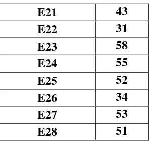
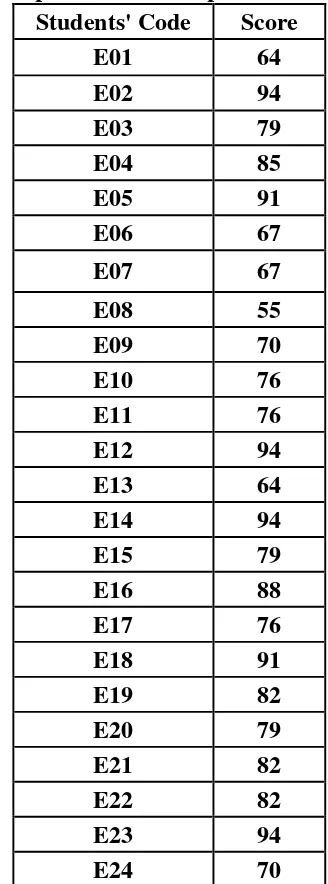
Table 4.5 The Description of Post Test Scores of The Data Achieved by The Students in Experimental Group
Students' Code Score
E01 64
E02 94
E03 79
E04 85
E05 91
E06 67
E07 67
E08 55
E09 70
E10 76
E11 76
E12 94
E13 64
E14 94
E15 79
E16 88
E17 76
E18 91
E19 82
E20 79
E21 82
E22 82
E23 94
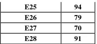
E25 94
E26 79
E27 70
E28 91
Based on the data above, it was known the highest score was 94 and the
lowest score was 55. To determine the range of score, the class interval, and
interval of temporary, the writer calculated using formula as follows:
The Highest Score (H) = 94 The Lowest Score (L) = 55
The Range of Score (R) = H – L + 1 = 94 – 55 + 1 = 40
The Class Interval (K) = 1 + (3.3) x Log n = 1 + (3.3) x Log 28 = 1 + (3.3) x 1.447158031 = 1 + 4.775621502
= 5.775621502 = 6
Interval of Temporary (I) =
6 40
K R
= 6,66666667 = 6 or 7
So, the range of score was 40, the class interval was 6, and interval of
temporary was 6. Then, it was presented using frequency distribution in the
following table:
Table 4.6 The Frequency Distribution of the Post Test Score of the Experimental Group
Class (k)
Interval (I)
Frequency (F)
Midpoint (X)
The Limitation
of Each Group
Relative Frequency
(%)
Cumulative Frequency
∑F = 28 ∑P = 100
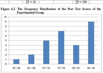
Figure 4.2. The Frequency Distribution of the Post Test Scores of the Experimental Group
The table and figure above shows the post test score of students in
experimental group. It could be seen that there was a student who got score 55 –
60. There were 2 students who got score 61 – 66. There were 5 students who got
score 67 – 72. There were 7 students who got 73 – 79. There were 4 students who
got 80 – 87 and there were 9 students who got 88 – 94. In this case, the treatment
was success make scores students’ vocabulary high and can see in the figure.
From 28 students, 9 students got higher score 88-94 and just a student got low
point 55-60.
The next step, the writer tabulated the score into the table for the calculation
of mean, median, and modus as follows:
0 1 2 3 4 5 6 7 8 9 10
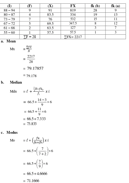
Table 4.7 The Calculation of Mean, Median, and Modus of the Post Test Scores of the Experimental Group
(I) (F) (X) FX fk (b) fk (a)
88 – 94 9 91 819 28 9
80 – 87 4 83.5 334 19 13
73 – 79 7 76 532 15 11
67 – 72 5 69.5 347.5 8 12
61 – 66 2 63.5 127 3 7
55 – 60 1 57.5 57.5 1 3
∑F = 28 ∑FX= 2217
a. Mean
Mx = ∑𝑓𝑋
𝑁
=
28 2217
=
79
.
17857
= 79.178b. Median Mdn = ℓ +
1 2𝑁−𝑓𝑘𝑏
𝑓𝑖 𝑥𝑖
= 6
9 3 14 5 .
66
= 6
9 11 5 .
66
=
66
.
5
7
.
333
=73
.
833
c. Modus
Mo = ℓ + 𝑓𝑎
𝑓𝑎+𝑓𝑏 𝑥𝑖
= 6
2 7
7 5 .
66
= 6
9 7 5 .
66
=
66
.
5
4
.
6666
The calculation above shows of mean value was 79.178, median value was
73.833, and modus value was 71.1666 of the post test of the experimental group.
The last step, the writer tabulated the scores of pre test of control group into
the table for the calculation of standard deviation and the standard error as
follows:
Table 4.8 The Calculation of the Standard Deviation and the Standard Error of the Post Test Scores of Experimental Group
(I) (F) (X) x’ Fx’ Fx’2
88 – 94 9 91 +3 27 81
80 – 87 4 83.5 +2 8 16
73 – 79 7 76 +1 7 7
67 – 72 5 69.5 0 0 0
61 – 66 2 63.5 -1 -2 2
55 – 60 1 57.5 -2 -2 4
∑F = 28 ∑Fx’ = 38 ∑Fx’2
= 110 a. Standard Deviation
N Fx N Fx i SD 2 2 1 ' '
2 1 28 38 28 110 6 SD 2 1 6 3.928(1.357)SD 8414 . 1 928 . 3 6
1
SD 0866 . 2 6 1 SD 4445 . 1 6
1
SD 667 . 8 1 SD
b. Standard Error
27 667 . 8
1
SEM
1961524227 .
5
667 . 8
1
SEM
6679649277 .
1
1
SEM
2
1
SEM
The result of calculation shows standard deviation of post test score of
experimental group was 8.667 and the standard error of post test score of
experimental group was 2.
The writer also calculated the data calculation of post-test score of
experimental group using SPSS 17.0 program. The result of statistic table is as
follows:
Table 4.9 The Frequency Distribution of the Post Test Scores of the Experimental Group Using SPSS 17.0 Program
Frequency Percent
Valid Percent
Cumulative Percent
Valid 55.00 1 3,6 3,6 3,6
64.00 2 7,1 7,1 10,7
67.00 2 7,1 7,1 17,9
70.00 3 10,7 10,7 28,6
76.00 3 10,7 10,7 39,3
79.00 4 14,3 14,3 53,6
82.00 3 10,7 10,7 64,3
85.00 1 3,6 3,6 67,9
88.00 1 3,6 3,6 71,4
91.00 3 10,7 10,7 82,1
94.00 5 17,9 17,9 100,0
Figure 4.3. The Frequency Distribution of the Post test Score of the Experimental Group Using SPSS 17.0 Program
The table and figure above shows the result of post-test scorer achieved by
the experiment group using SPSS Program. It could be seen that there was a
student who got 55 (3.6%). Two student got 64 (7.1%). Two students got 67
(7.1%). Three students got 70 (10.7%). Three students got 76 (10.7%). Four
students got 79 (14.3%). Three students got 82 (10.7%). One student got 85
(3.6%). One student got 88 (3.6%). Three students got 91 (10.7%). Five students
got 94 (17.9%).
The next step, the writer calculated the score of mean, median, mode,
standard deviation, and standard error of mean of post-test score in experiment
group as follows:
The Frequency Of Post Test in Experiment Group
Table 4.10 The Table of Calculation of Mean, Median, Mode, Standard Deviation, and Standard Error of Mean of Post-test Score in Experiment Group Using SPSS 17.0 Program
N Valid 28
Missing 0
Mean 79,7500
Std. Error of Mean 2,07952
Median 79,0000
Mode 94,00
Std. Deviation 11,00379
Variance 121,083
Range 39,00
Minimum 55,00
Maximum 94,00
Sum 2233,00
The table shows the result of mean calculation was 79,7500, the result of
median calculation was 79,0000, and the result of mode calculation was 94,00.
The result of standard deviation calculation was 11,00379 and the result of
standard error of mean calculation was 2,07952.
2. Distribution of the Control Group Scores
a. Distribution of Pre Test Scores of the Control Group
The pre test scores of the control group were presented in the following
table.
Table 4.11 The Description of Pre Test Scores of The Data Achieved by The Students in Control Group
Students' Code Score
C01 37
C03 31
C04 43
C05 34
C06 55
C07 49
C08 58
C09 34
C10 43
C11 55
C12 31
C13 64
C14 49
C15 55
C16 43
C17 55
C18 67
C19 34
C20 43
C21 34
C22 40
C23 43
C24 61
C25 43
C26 46
C27 64
C28 61
C29 55
Based on the data above, it was known the highest score was 67 and the
lowest score was 31. To determine the range of score, the class interval, and
interval of temporary, the writer calculated using formula as follows:
The Highest Score (H) = 67 The Lowest Score (L) =31
The Class Interval (K) = 1 + (3.3) x Log n = 1 + (3.3) x Log 29
= 1 + (3.3) x 1.4623979979 = 1 + 4.8259133931
= 5.8259133931 = 6
Interval of Temporary (I) =
6 40
K R
= 6,66666667 = 6
So, the range of score was 40, the class interval was 6, and interval of
temporary was 6. Then, it was presented using frequency distribution in the
following table:
Table 4.12 The Frequency Distribution of the Pre Test Score of the Control Group
Class (k)
Interval (I)
Frequency (F)
Midpoint (X)
The Limitation
of Each Group
Relative Frequency
(%)
Cumulative Frequency
(%) 1 61 – 67 5 64 60.5 – 67.5 17,241 100
2 55 – 60 6 57.5 54.5 – 60.5 20,690 82,759
3 49 – 54 3 51.5 48.5 – 54.5 10,345 62,069
4 43 – 48 7 45.5 42.5 – 48.5 24,138 51,724
5 37 – 42 2 39.5 36.5 – 42.5 6,897 27,586
6 31 – 36 6 33.5 30.5 – 36.5 20,690 20,690
∑F = 29 ∑P = 100
Figure 4.4. The Frequency Distribution of the Pre Test Scores of the Control Group
0 1 2 3 4 5 6 7 8
The table and figure above shows the pre test score of students in
experimental group. It could be seen that there were 6 students who got score 31 –
36. There were 2 students who got score 37 – 42. There were 7 students who got
score 43 – 48. There were 3 students who got 49 – 54. There were 6 students who
got 55 – 60 and there were 5 students who got 61 – 67. In this case, so many
students got point 43-48 and some students got point 61-67 in the pretest. The
next step, the writer tabulated the score into the table for the calculation of mean,
median, and modus as follows:
Table 4.13 The Calculation of Mean, Median, and Modus of the Pre Test Scores of the Control Group
(I) (F) (X) FX fk (b) fk (a)
61 – 67 5 64 320 29 5
55 – 60 6 57.5 345 24 11
49 – 54 3 51.5 154,5 18 9
43 – 48 7 45.5 318,5 15 10
37 – 42 2 39.5 79 8 9
31 – 36 6 33.5 201 6 8
∑F = 29 ∑FX= 1418
a. Mean
Mx = ∑𝑓𝑋
𝑁
=
29 1418
=
48
.
8965517
= 48.896b. Median Mdn = ℓ +
1 2𝑁−𝑓𝑘𝑏
𝑓𝑖 𝑥𝑖
= 6
5 8 5 . 14 5 .
42
= 6
5 5 . 6 5 .
=
42
.
5
7
.
8
=50
.
3
c. Modus
Mo = ℓ + 𝑓𝑎
𝑓𝑎+𝑓𝑏 𝑥𝑖
= 6
2 3
3 5 .
42
= 6
5 3 5 .
42
=
42
.
5
3
.
6
=
46
.
1
The calculation above shows of mean value was 48.896, median value was
50.3, and modus value was 46.1 of the post test of the control group.
The last step, the writer tabulated the scores of pre test of control group into
the table for the calculation of standard deviation and the standard error as
follows:
Table 4.14 The Calculation of the Standard Deviation and the Standard Error of the Post Test Scores of Control Group
(I) (F) (X) x’ Fx’ Fx’2
61 – 67 5 64 +3 15 45
55 – 60 6 57.5 +2 12 24
49 – 54 3 51.5 +1 3 3
43 – 48 7 45.5 0 0 0
37 – 42 2 39.5 -1 -2 2
31 – 36 6 33.5 -2 -12 14
∑F = 29 ∑Fx’ = 16 ∑Fx’2
= 98
a. Standard Deviation
2 1 6 3.379(0.5517)
SD 30437 . 0 379 . 3 6
1
SD 07463 . 3 6 1 SD 753 . 1 6
1
SD 518 . 10 1 SD
b. Standard Error
1 1 1 1 N SD SEM 1 29 518 . 10 1 SEM 28 518 . 10 1 SEM 2915 . 5 518 . 10 1 SEM 98771 . 1 1 SEM 987 . 1 1 SEM
The result of calculation shows the standard deviation of pre test score of
control group was 10.518and the standard error of post test score of experimental
group was 1.987.
b. Distribution of Post Test Scores of the Control Group
The post test scores of the control group were presented in the following
table.
Table 4.15 The Description of Post Test Scores of The Data Achieved by The Students in Control Group
Students' Code Score
C01 40
C02 55
C03 37
C05 40
C06 49
C07 64
C08 67
C09 40
C10 40
C11 64
C12 64
C13 94
C14 67
C15 73
C16 70
C17 76
C18 58
C19 31
C20 31
C21 58
C22 88
C23 31
C24 67
C25 52
C26 94
C27 82
C28 58
C29 67
Based on the data above, it was known the highest score was 94 and the
lowest score was 31. To determine the range of score, the class interval, and
interval of temporary, the writer calculated using formula as follows:
The Highest Score (H) = 94 The Lowest Score (L) =31
The Range of Score (R) = H – L + 1 = 94 – 31 + 1 = 64
The Class Interval (K) = 1 + (3.3) x Log n = 1 + (3.3) x Log 29
= 5.8259133931 = 6
Interval of Temporary (I) =
6 64
K R
= 10.666666667 =10 or 11
So, the range of score was 70, the class interval was 6, and interval of
temporary was 10. Then, it was presented using frequency distribution in the
following table:
Table 4.16 The Frequency Distribution of the Pos Test Scores of the Control Group
Class (k)
Interval (I)
Frequency (F)
Midpoint (X)
The Limitation
of Each Group
Relative Frequency
(%)
Cumulative Frequency
(%) 1 83 – 94 3 88.5 62.5 – 94.5 10,345 100
2 72 – 82 3 77 71.5 – 82.5 10,345 6,897
3 61 – 71 8 66 60.5 – 71.5 27,586 -3,448
4 51 – 60 5 55.5 50.5 – 60.5 17,241 0,000
5 41 – 50 2 45.5 40.5 – 50.5 6,897 82,759
6 31 – 40 8 35.5 30.5 – 40.5 27,586 -6,897
∑F = 29 ∑P = 100
Figure 4.5. The Frequency Distribution of the Post test Score of the Control Group
0 1 2 3 4 5 6 7 8 9
The table and figure above shows the post test score of students in control
group. It could be seen that there were 8 students who got score 31 – 40. There
ware 2 students who got score 41 – 50. There were 5 students who got score 51 –
60. There were 8 students who got 61 – 71. There ware 3 students who got 72 –
82 and there were 3 students who got 83 - 94. From the chart can see the scores of
post test many students got less scores 31-40, that is same with the average
scores61-71. That give proof with English song media, students’ vocabulary will
increase. The next step, the writer tabulated the scores into the table for the
calculation of mean, median, and modus as follows:
Table 4.17 The Calculation of Mean, Median, and Modus of the Post Test Scores of the Control Group
(I) (F) (X) FX fk (b) fk (a)
83 – 94 3 88.5 265.5 29 3
72 – 82 3 77 231 26 6
61 – 71 8 66 528 23 11
51 – 60 5 55.5 277.5 15 13
41 – 50 2 45.5 91 10 7
31 – 40 8 35.5 284 8 10
∑F = 29 ∑FX= 1767
a. Mean
Mx = ∑𝑓𝑋
𝑁
=
29 1767
= 60.9310344828 = 60.931
b. Median Mdn = ℓ +
1 2𝑁−𝑓𝑘𝑏
𝑓𝑖 𝑥𝑖
= 10
3 10 5 . 14 5 .
50
= 10
3 5 . 4 5 .
50
=
50
.
5
15
c. Modus
Mo = ℓ + 𝑓𝑎
𝑓𝑎+𝑓𝑏 𝑥𝑖
= 10
2 8
8 5 .
50
= 10
10 8 5 .
50
=
50
.
5
8
=
58
.
5
The calculation above shows of mean value was 60,931, median value was
65.5 and modus value was 58.5 of the pre test of the control group. The last step,
the writer tabulated the scores of pre test of control group into the table for the
calculation of standard deviation and the standard error as follows:
Table 4.18 The Calculation of the Standard Deviation and the Standard Error of the Pre Test Scores of Control Group
(I) (F) (X) x’ Fx’ Fx’2
83 – 94 3 88.5 +2 6 12
72 – 82 3 77 +1 3 3
61 – 71 8 66 0 0 0
51 – 60 5 55.5 -1 -5 5
41 – 50 2 45.5 -2 -4 8
31 – 40 8 35.5 -3 -24 72
∑F = 29 ∑Fx’ = -24 ∑Fx’2 = 100
a. Standard Deviation
N Fx N Fx i SD 2 2 1 ' '
2 1 29 24 29 100 10 SD 2 1 10 3.448(0.82758)SD 684888 . 0 448 . 3 10
1
SD 763112 . 2 10 1 SD 6622 . 1 10
1
SD 622 . 16 1 SD
b. Standard Error
1 29
622 . 16
1
SEM
28 622 . 16
1
SEM
291 . 5
622 . 16
1
SEM
141 . 3
1
SEM
The result of calculation shows the standard deviation of post test score of
control group was 16,622 and the standard error of post test score of control group
was 3,141.
The writer also calculated the data calculation of post-test score of
experimental group using SPSS 17.0 program. The result of statistic table is as
follows:
The writer also calculated the data calculation of post-test score of experimental
group using SPSS 17.0 program. The result of statistic table is as follows:
Table 4.19 The Frequency Distribution of the Post Test Scores of the Control Group Using SPSS 17.0 Program
Frequency Percent
Valid Percent
Cumulative Percent
Valid 31.00 3 12,5 12,5 12,5
37.00 1 4,2 4,2 16,7
40.00 4 16,7 16,7 33,3
46.00 1 4,2 4,2 37,5
49.00 1 4,2 4,2 41,7
55.00 1 4,2 4,2 45,8
58.00 2 8,3 8,3 54,2
64.00 3 12,5 12,5 66,7
67.00 3 12,5 12,5 79,2
70.00 1 4,2 4,2 83,3
73.00 1 4,2 4,2 87,5
76.00 1 4,2 4,2 91,7
94.00 1 4,2 4,2 100,0
Total 24 100,0 100,0
Figure 4.6. The Frequency Distribution of the Post test Score of the Control Group Using SPSS 17.0 Program
The table and figure above shows the result of post-test scorer achieved by
the control group using SPSS Program. It could be seen that there were 3 students
who got 31 (12.5%). One student got 37 (4.2%). Four students got 40 (16.7%).
One student got 46 (4.2%). One student got 49 (4.2%). One student got 55 (4.2%).
Two students got 58 (8.3%). Three students got 64 (12.5%). Three students got 67
(12.5%). One student got 70 (4.2%). One student got 73 (4.2%). One student got
76 (4.2%). One student got 88 (4.2%). And one student got 94 (4.2%).
The next step, the writer calculated the score of mean, median, mode,
standard deviation, and standard error of mean of post-test score in experiment
group as follows:
The Frequency Of Post Test in Control Group
Table 4.20 The Table of Calculation of Mean, Median, Mode, Standard Deviation, and Standard Error of Mean of Post-test Score in Experiment Group Using SPSS 17.0 Program
N Valid 24
Missing 0
Mean 56,2500
Std. Error of Mean 3,64267
Median 58,0000
Mode 40,00
Std. Deviation 17,84535
Variance 318,457
Range 63,00
Minimum 31,00
Maximum 94,00
Sum 1350,00
The table shows the result of mean calculation was 56,2500, the result of
median calculation was 58,0000, and the result of mode calculation was 40,00.
The result of standard deviation calculation was 17,84535 and the result of
standard error of mean calculation was 3,64267.
B. The Result of Data Analysis
1. Testing Hypothesis Using Manual Calculation
The writer chose the significance level on 5%, it means the significant level
of refusal of null hypothesis on 5%. The writer decided the significance level at
5% due to the hypotheses type stated on non – directional ( two – tailed test ). It
meant that the hypothesis can’t direct the prediction of alternative hypothesis.
answer of hypothesis, “1” can be ( > ) or ( < ). The answer of hypothesis could not
be predicted whether on more than or less than.
To test the hypothesis of the study, the writer used t-test statistical
calculation. Firstly, the writer calculated the standard deviation and the standard
error of X1 and X2. It was found the standard deviation and the standard error of
post test of X1 and X2 at the previous data presentation. It could be seen on this
following table.
Table 4.21 The Standard Deviation and the Standard Error of X1 and X2 Variable The Standard Deviation The Standard Error
X1 11,00379 2,07952
X2 17,84535 3,64267
Where:
X1 = Pre test of experiment group
X2 = Post test of experiment group
The table shows the result of the standard deviation calculation of X1 was
11,00379 and the result of the standard error mean calculation was 2,07952. The
result of the standard deviation calculation of X2 was 17,84535 and the result of
the standard error mean calculation was 3,64267.
The next step, the writer calculated the standard error of the differences
mean between X1 and X2 as follows:
Standard Error of Mean of Score Difference between Variable I and Variable II
2 1 M M SE
SE = 2
2 2
1 M
M SE
SE
2 1 M M SE
SE = 2 2
3,64267 2,07952
2 1 M M SE
2 1 M M SE
SE = 8.9446
2 1 M M SE
SE =
2
.
99705
2 1 M M SE
SE =
2
.
997
The calculation above shows the standard error of the differences mean
between X1 and X2 was 2.997. Then, it was inserted to the to formula to get the
value of t observe as follows:
o
t =
2 1
2 1
M M SE
SE M M
o
t =
2.997 56,2500 79,7500
o
t =
2.997 5 , 23
o
t =
7
.
8411
With the criteria:
If t-test (t-observed) ≥ ttable,it means Ha is accepted and Ho is rejected.
If t-test (t-observed) < ttable,it means Ha is rejected and Ho is accepted.
Then, the writer interpreted the result of t- test. Previously, the writer
accounted the degree of freedom (df) with the formula:
df = (N1 N2 2) = (28292)
=
55
table
t at df 58/60 at 5% significant level = 2.000
The writer chose the significance level on 5%, it means the significant level
of refusal of null hypothesis on 5 %. The writer decided the significance level at
meant that the hypothesis can not direct the prediction of alternative hypothesis.
Alternative hypothesis symbolized by ”1”. This symbol could not direct the
answer of hypothesis, “1” can be ( > ) or ( < ). The answer of hypothesis could not
be predicted whether on more than or less than
The calculation above shows the result of t-test calculation as in the table
follows:
Table 4.22 The Result of T-test
Variable t observe t table Df/db
5% 1%
X1- X2 10.883 2.000 2.660 55
Where:
X1 = Pre Test
X2 = Post Test
t observe = The calculated Value
t table = The distribution of t value
df/db = Degree of Freedom
Based on the result of hypothesis test calculation, it was found that the value
of tobserved was greater than the value of table at 1% and 5% significance level or
2.000 < 10.883 > 2.660. It meant Ha was accepted and Ho was rejected.
It could be interpreted based on the result of calculation that Ha stating that
song gives effect on the students’ vocabulary score was accepted and Ho stating
that song does not give effect on the students’ vocabulary score was rejected. It
vocabulary score of the seventh grade students at MTs Darul Amin of Palangka
Raya.
2. Testing Hypothesis Using SPSS Calculation
The writer also applied SPSS 17.0 program to calculate t test in testing
hypothesis of the study. The result of the t test using SPSS 17.0 was used to
support the manual calculation of the t test. The result of the t test using SPSS
17.0 program could be seen as follows:
Table 4.23 The Standard Deviation and the Standard Error of X1 and X2 Group Statistics
VAR00001 N Mean
Std.
Deviation
Std. Error
Mean
VAR00002 1.00 28 79,7500 11,00379 2,07952
2.00 29 58,7241 18,29500 3,39730
The table shows the result of the standard deviation calculation of X1 was
11,00379 and the result of the standard error mean calculation was 2,07952. The
result of the standard deviation calculation of X2 was 17,84535 and the standard
Table 4.24 The Calculation of T-test Using SPSS 17.0
The table shows the result of t-test calculation using SPSS 17.0 program.
Since the result of post-test between experiment and control group had difference
score of variance, it meant the t-test calculation used at the equal variances not
assumed. It found that the result of tobserved was 5.279, the result of mean
difference between experiment and control group was 21,02586, and the standard
error difference between experiment and control group was 3,98322.
To examine the truth or the false of null hypothesis stating that song does
not give effect on the students’ vocabulary score, the result of t-test was
interpreted on the result of degree of freedom to get the table. The result of degree
of freedom (df) was 55, it found from the total number of the students in both Table 4.24 Independent Samples Test
Levene's Test for Equality of
Variances
t-test for Equality of Means
F Sig. T Df
S ig. (2-taile d ) M ean Diff er en ce S td. E rr or Diff er en
ce Confidence 95% Interval of the Difference L owe r Upp er VA R00002 Equal variances assumed 6,69 9
,012 5,2 35
55 ,000 21,0 2586 4,0 16 70 12,9 7621 29,0 7551 Equal variances not assumed 5,2 79 46, 18 9
group minus 2. The following table was the result of tobserved and table from 55 df at
5% and 1% significanc5e level.
Table 4.25 The Result of T-test Using SPSS 17.0
Variable t observe t table Df/db
5% 1%
X1- X2 5,279 2.000 2.660 55
The interpretation of the result of t-test using SPSS 17.0 program, it was
found the t observe was greater than the t table at 1 % and 5 % significance level
or 2.000< 5,279>2.660. It meant Ha was accepted and Ho was rejected.
It could be interpreted based on the result of calculation that Ha stating that
song gives effect on the students’ vocabulary score was accepted and Ho stating
that English song does not give effect on the students’ vocabulary score was
rejected. It meant that teaching vocabulary with English song gave significant
effect on the students’ vocabulary score of the seventh grade students at MTs
Darul Amin of Palangka Raya.
3. Normality and Homogeneity test
Best on post test, the writer make a normality test and homogeneity test to
analyzed whether both group with SPSS 17.0.
a. Normality Test
4.26 Case Processing Summary
Cases
Valid Missing Total
N Percent N Percent N Percent
Control 28 93,3% 2 6,7% 30 100,0%
The table show the result of processing in the test is 93% is valid and for
missing just 6,7%.
4.27 The Calculation of Tests of Normality Using SPSS 17.0 Kolmogorov-Smirnov
a
Shapiro-Wilk
Statistic df Sig. Statistic df Sig.
Control ,125 28 .200* ,954 28 ,247
Experiment ,132 28 .200* ,938 28 ,099
The table shows the result of calculating of test of normality test, the
significant of control group 0.247 and experiment group 0,099. So the test is
normal because value of normality is p > 0,005 the test is normality.
b. Homogeneity Test
4.28 The Result of Test of Homogeneity of Variances Using SPSS 17.0 Experiment
Levene Statistic df1 df2 Sig.
1.025 5 12 .446
The table shows the result of calculating of test of homogeny test, the
significant of experiment group 0,0446. The test is homogeny because value of
homogeny is p > 0,005 the test is homogeny.
C. Discussion
The result of the data analysis shows that English song gave significant
effect on the students’ English vocabulary at the seventh graders of MTs Darul
Amin Palangka Raya. The result of post test be higher than the result of pre test
after were taught using English song. It was also proved by the result of
the value of table at 1% and 5% significance level or 2.000 < 5.279 > 2.660. It
meant Ha was accepted and Ho was rejected.
Furthermore, the result of t-test calculation using SPSS 17.0 also shows
that using English song in taught English vocabulary gave significant effect on the
students’ English vocabulary score. It was proved by the mean score pre test of
the students before were taught using English song got 45.17 and post test score
of the students after were taught using English song got 73.833. It was also proved
by the value of tobserve was greater than the value of ttable both at 1% and 5%
significance level or 2.021< 5.279 >2.704. It meant Ha was accepted and Ho was
rejected.
The findings of the study based on the result of manual and SPSS 17.0
program calculation could be interpreted that the alternative hypothesis stating
that teaching English vocabulary by using English song gives effect on the
students’ vocabulary score of the seventh graders of MTs Darul Amin Palangka
Raya was.
The findings of the study verified the theories of English song as a
beneficial and a good strategy for English vocabulary (Chapter II, pg.27). First of
all, English song can increase the students’ vocabulary score. It can be seen from
the difference between students’ score in the pretest and post test.
In this case, English song is one of suitable strategy for the students to help
them in the process of English vocabulary with the goal of improving some
aspects of skill, because the use of English song can motivating and challenging
II, pg.26). It can be seen from the difference between students’ number of