DOI: 10.12928/TELKOMNIKA.v13i1.1263 221
Received Signal Strength Indicator Node Localization
Algorithm Based on Constraint Particle Swarm
Optimization
Songhao Jia*, Cai Yang
Department of Computer and Information Technology, Nanyang Normal University, Nanyang 473061, Henan, China
*Corresponding author, e-mail: [email protected]
Abstract
Because the received signal strength indicator (RSSI) value greatly changes, the direct use of RSSI value has more errors in the positioning process as the basis to calculate the position of anchor nodes. This paper proposes a RSSI node localization algorithm based on constraint particle swarm optimization (PSO-RSSI). In the algorithm, particle swarm optimization is used to select anchor nodes set which are near the unknown node. The algorithm takes an element in the set, and measure distance between it and the other elements in the set. Then, the maximum likelihood method is used to calculate the coordinates. According to the difference between the calculated coordinates and the actual coordinates of the anchor node, the obtain coordinate of unknown node is corrected. When all the elements in the set perform such operation, the statistical methods are used to determine the coordinates of the unknown node. The algorithm embodies all the reference points influence on positioning, corrects the error problem on a single reference node positioning in the past. The simulation results show that the effect of the PSO-RSSI algorithm is more excellent.
Keywords: constraint particle swarm optimization, wireless sensor network, RSSI algorithm, node localization
1. Introduction
With the rapid development of integrated circuit, sensor and wireless network technology, Wireless Sensor Networks (WSN) are more and more concerned by all the countries in the world. Wireless sensor network is mainly composed of the sensor node, the sink node and monitoring center, has the information processing and information communication function. Obtain accurate location information of sensor nodes and transmit them to the control center, is critical for WSN. According to whether need ranging, positioning algorithms are divided into range based localization algorithm (Range-based) and range free localization algorithm (Range-free). The Range-based algorithm measures distance or range parameters of unknown node to locate. It has the advantage of high positioning accuracy, but requires additional hardware support. The Range-free algorithm only depends on the connectivity of the network to achieve the positioning. Compared with the Range-based algorithm, this algorithm has the relatively small power consumption, and the positioning accuracy is lower than the former calculation. Because the above two types of localization algorithms have advantages and disadvantages, people care about energy consumption and precision positioning and hope to get the best service at minimum cost.
the authors use the Interdisciplinary Institute for Broadband Technology real-life test bed and present an automated method to optimize and calibrate the experimental data before offering them to a positioning engine. In a preprocessing localization step, they introduce a new method to provide bounds for the range, thereby further improving the accuracy of our simple and fast 2D localization algorithm based on corrected distance circles [3]. Byoungsu Lee and Seungwoo Kim developed the design technology of a sensing platform for the HWR to perform a role of both health and life care in an aging society. A fusion algorithm using RSSI and trilateration is also proposed for the agile self-localization [4]. Gaddi Blumrosen et al proposed a new tracking system based on exploitation of Received Signal Strength Indicator measurements in WSN. The system is evaluated in indoor conditions and achieves tracking resolution of a few centimeters which is compatible with theoretical bounds [5]. A.LAKSHMI et al proposed novel energy efficient algorithm FDPCA for Wireless Sensor Networks. Parameters like End to End Delay and Received Signal Strength Indicator are considered for exercising the influence on transmit power. The proposed algorithm can effectively save energy without degrading the throughput of the network and reduce the energy consumption of the network [6].Those documents put forward the improvement measures of the RSSI algorithm, but these methods can only reduce the effects of transient disturbance. Moreover, the positioning accuracy is not high, the efficiency is low.
Aiming at these problems, based on the analysis of the traditional RSSI positioning algorithm, this paper proposes RSSI node localization algorithm based on constraint particle swarm optimization. Because the particle swarm optimization algorithm can iterative search the optimal solution, it is used to find neighboring nodes set of the unknown node, which meet certain conditions or threshold. The nodes in the set are used to assist localization of unknown node. Select a node in the set as the reference node, other nodes in the set are used to measure its location by the RSSI algorithm. Comparison of actual coordinate reference node, the error value is written down. By using the same method, the coordinates of unknown node is calculated. Then, the error values of reference node are used to modify coordinates of the unknown node. When all the nodes in the set perform the operation, the coordinates of unknown node are calculated by using statistical method. The algorithm does not need additional hardware, due to the introduction of particle swarm algorithm, improves the efficiency and accuracy of positioning. The simulation results show that the PSO-RSSI algorithm is more
accurate, and it has less error and better performance.
2. The Algorithm Model
2.1. Particle swarm optimization algorithm
Particle swarm optimization algorithm is a kind of evolutionary algorithm for global optimization. Inspired by the birds of prey behavior, Dr R.Eberhart and Dr J.Kennedy proposed the algorithm. In the optimization problem and nonlinear processing combination optimization problem, particle swarm optimization algorithm has very good effect [7]-[9].
2.1.1. The principle of particle swarm optimization algorithm
Particle swarm optimization algorithm is a stochastic particle swarm, and each particle in the particles population finds its optimal solution by iteration method process. Assume that in a D target search space, a community composed of M particles. D dimensional vector said one of the particles. As shown in equation (1).
1 2
( , ), 1, 2
i i i iD
x x x x i m (1)
xi said target location of the particle i in the D dimension search space. In the D dimension search space, each particle position is a potential solution, also may be the optimal solution. Through put xi into the objective function, the adaptation values can be calculated, and measure the merits of xi by the fitness value. Assuming vi=( vi1, vi2 …viD) is the speed of particle i. pi=( pi1, pi2 …piD) is the optimal position of the particle i. pg=( pg1, pg2 …pgD) is the best position of particle swarm so far to search.
k+1 k k k and the effect more than 4 or less than 0 optimization algorithms is not very good. Learning factors is used to guide and promote the optimal particle to the optimal value and the entire population of all particles [10, 11].
(2) r1, r2 is a number of random distribution value from 0 to 1.
2.1.2. Process of particle swarm optimization algorithm
The standard particle swarm optimization procedure is as follows: Step 1 : Initialize the particle population.
Step 2 : Adaptive value of each particle is calculated.
Step 3 : According to the value of each particle calculated in Step 2, their individual optimal solution is updated. At the same time, the optimal solution of group is found, and the index value is stored.
Step 4 : Using the formula (2) and formula (3), speed and position of each particle are recalculated.
Step 5 : Judge whether the fitness value reaches the predetermined requirements or the maximum number of iterations is reached, if met, then end the iteration. Otherwise, Step 2 is turned.
2.2. The maximum likelihood estimation method
Suppose node p1(x1, y1), p2(x2, y2), p3(x3, y3)…pn(xn, yn) is the anchor node. M(x, y) is the unknown node. d1, d2, d3…dn is expressed as the distance between anchor node and the unknown node M. According to the geometric knowledge, the following equation formula can be obtained.
In the formula (4), the first equations, the second equations...the n-1 equations sequentially minus the n equations, draw the following equation formula.
2 2 2 2 2 2
The equation, X= (ATA)-1ATb, is draw. According to this equation, the unknown node location of M can be calculated.
2 2 2 2 2 2
(1) RSSI values of all nodes in WSN are collected, and the RSSI values are converted to the distance
With the increase of distance, wireless signal will be regularly attenuated. This attenuation has great influence on the positioning accuracy of RSSI. So we should choose a suitable attenuation model of wireless signal. The commonly used wireless channel propagation attenuation model includes Free Space Propagation Model (Free-Space Model) and Log-distance Distribution Model [12],[13].
The Free-Space model is shown in formula (8):
)
Wherein, Loss represents the channel attenuation (unit: dB), d said the distance between the test point and source distance (unit: km), f represents the signal frequency (unit: MHz), k said attenuation factor.
Because of the signal interference and the obstacle factors, the Log-distance Distribution model is often used to determine the relationship between signal strength and distance. The Log-distance Distribution model is shown in formula (9):
In formula (9), d represents the distance between the current node and the source node. PL(d) is the path loss at the receiving node. Xσ said Gauss distributed random variables, the average value of which is 0. The range of it is 4~10. k represents the attenuation factor, in different circumstances, its value is different, which range is 2~5.
Generally, known transmit node's signal strength, the receiving node's signal strength and the gain of the antenna, using formula (10) can get the channel attenuation value.
RSSI P G-PL (d) (10)
In formula (10), P represents transmit power, G said antenna gain. By formula (10), PL(d) can be obtained. d0 is the reference distance, usually is taken as 1m. Putting it into formula (8), PL(d0) can be obtained. Putting PL(d) and PL(d0) into the formula (9) can get the required distance d.
(2) The introduction of particle swarm optimization algorithm
Particle swarm algorithm is a process of finding the particles optimal solution through constant iterations. The current optimal values are used to find the global optimum. Based on the particle swarm algorithm, the anchor nodes are obtained, which are near around the unknown node. These anchor nodes form a set. Because the nodes in WSN are random release, this will cause some particles random moving around, not to get the fastest way to find optimal solution. In order to avoid the occurrence of such a situation, restrictive conditions are added, and the course of finding the optimal solution is improved. In the comparison process, the improved method releases the nodes which are far from the optimal solution. By reducing the times of comparison, the iterative amount is reduced [14]-[16].
Specific steps are as follows:
Step l: initialization parameters of PSO.
2 i ri iF
f d(11)
Among them, fi
xix
2 yiy
2 .Step 3: Comparison of the calculated particle solution with the respective optimal solutions, the best solution is found. By comparison, better value are updated and replaced. Save the current best value of the optimal traversal, continue to repeat, the global optimal solution are found in the whole population.
Step 4: When the condition is reached (arrived at the threshold or the traversal is completed), the algorithm is end. All solutions are sorted, and the optimal approaching node set is obtained.
(3) Calculating the coordinates of the unknown node
Each anchor node of the set is taken out, and its positioning is measured by other anchor nodes in the set. Then, the maximum likelihood method is used to calculate the coordinates of the anchor node. Comparison with the actual coordinates, the error value is obtained. The unknown node is located by using the same method, the coordinate value is obtained. According to the error value of anchor nodes, the obtained coordinates of unknown node are corrected. This recursion, all the elements in the set performs the same operation, until the elements in the collection traversal is completed. Finally, the method of statistics is used to calculate the final coordinates of the unknown node [17]-[19].
3.2. The algorithm implementation process
Based on the above proposed algorithms, the implementation steps are as follows: Step 1: Anchor nodes periodically send its information to other node within the communication scope. This information includes ID number, Coordinate position information and so on. Each node spreads in turn.
Step 2: According to different anchor nodes, the unknown node classifies the received information. When the received signal exceeds a certain threshold, the average value of same anchor node RSSI is calculated.
Step 3: According to RSSI from strong to weak order, the mapping of RSSI value and the distance between unknown node and the anchor node is established. Particle swarm optimization algorithm is used to derive a set of anchor nodes adjacent to the unknown node.
The anchor node set: B_set = {b1, b2, …, bm}
Step 4: Select an anchor node in the set, the distance is measured by the other elements in the set. Then, the maximum likelihood method is used to calculate its coordinates (xi, yi). Compared with the actual coordinates (xri, yri), obtained the error value △xi(△xi=xri-xi), △yi(△yi=yri-yi).
Step 5: The coordinates of the unknown node are obtained by the same method, expressed as: (x, y). According to the error value from step 4, the coordinate (x, y) is corrected. Then, the coordinates is obtained, expressed as: (xui, yui). Among them, xui=x+△xi,yui=y+△yi .
Step 6: Another element in the set is taken to do step (4), until a collection iterates over. Step 7: According to the obtained coordinate value of the unknown node, the method of statistics is used to calculate the finally coordinate value of it. The coordinates of the unknown node is expressed as the average value.
4. The Simulation Results and Analysis
4.1. The algorithm implementation process
In order to better test the performance of the new algorithm, in the simulation of the actual environment, wireless sensor network nodes randomly deployed in a network region [20],[21].
The experimental parameter settings are as follows:
(1) The range of measured region: the square area of 100m * 100m
(2) The total number of nodes is 100. Among them, the anchor nodes are respectively 10, 15, 20, 25, 30, 35, 40, 45, and 50. The positions of the unknown nodes are randomly generated by MATLAB 2012. The simulation runs 100 times.
(3) Communication radius: Communication radius of node is 10-100m; the starting value is set 50m.
(4) The simulation experiment using the shadowing model which has reference distance d0=1 and P (d0) = -40.
(5) Gaussian distribution variance xσ=2.
All the simulation data are average values, obtained through many simulations.
Node relative positioning error can be represented by the deviation of estimating the position and the actual location. As shown in formula (12):
% estimated node position information, R said node communication radius.
The average localization error rate is expressed as all nodes average error rate. As shown in formula (13):
Among them, n represents the numbers of unknown nodes, δ said network average localization error rate.
4.2. Influencing Factors
The performances of two algorithms on the location error are observed through number of anchor nodes, total number of nodes and communication radius. In order to improve the simulation accuracy, this paper uses statistical methods. The following are 100 measurement results.
(1) Effects of number of anchor nodes on positioning precision
Figure 1. Effects of number of anchor nodes on positioning precision
Figure 1 shows that, in the whole wireless sensor network, the total number of nodes are fixed, the change of anchor nodes have certain degree of influence on the positioning error. Overall, with the increase in the number of anchor nodes, the positioning accuracy of the traditional RSSI algorithm and the PSO-RSSI algorithm corresponding increase, and the error is reduced. Comparing the two curves in the Figure 1, in the process of increased from 10 to 50 anchor nodes, the PSO-RSSI algorithm is better than the orientation of the common RSSI algorithm with high accuracy and low error. This show that the PSO-RSSI algorithm improves positioning accuracy, reduce the positioning error function.
But more than a certain range, this setting is not too large role. This shows that positioning error change is not obvious, when anchor nodes are added to a certain number. This time, location error is not reducing by simply increasing the number of anchor nodes.
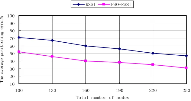
(2) Effects of total number of nodes on positioning precision
In the condition of unchanged of the anchor nodes proportion and the total number of nodes increases, the performance of the two algorithms performance are as shown in Figure 2. With the number of nodes increases, it is can be seen from the Figure 2 that the positioning errors of the two algorithms show a downward trend. Under the same conditions, the average positioning error of PSO-RSSI algorithm is far less than the original RSSI algorithm. With the increase of the number of nodes, node distribution is more uniform and reasonable, which reduces the influence on the accuracy of positioning.
Figure 2. Effects of total number of nodes on positioning precision
0 1 2 3 4 5 6 7
10 15 20 25 30 35 40 45 50
number of anchor nodes
The positioning error/
m
RSSI PSO-RSSI
10 20 30 40 50 60 70 80 90 100
100 130 160 190 220 250
Total number of nodes
The a
verag
e pos
ition
ing e
rror
%
(3) Effects of communication radius on positioning precision
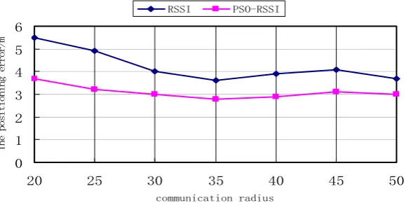
The greater the radius of communication nodes, covering more anchor nodes, and vice versa. Therefore, by changing the radius of communication, its effect is observed on the algorithm of average positioning error. In this experiment, the number of anchor nodes is a fixed value of 20, the other parameters are constant, and the communication radius is the only change quantity. Communication radius from 20m according to 5m each step until the communication radius of 50m, the effect of node communication radius on the algorithm of error is observed. The result is shown in Figure 3.
Figure 3. Effects of communication radius on positioning precision
It is shown that the communication radius is too large or too small will affect the positioning error. When communication radius is 35 meters, the positioning error is smallest. Therefore, according to the situation in practical application, the appropriate sensors are selected. Under the same conditions, the average localization error of the PSO-RSSI algorithm is significantly less than the RSSI algorithm, the positioning accuracy is significantly improved. This shows that the new algorithm has better performance.
To sum up, by changing number of anchor nodes, total number of nodes and communication radius, performance of PSO-RSSI algorithm is better than the original RSSI algorithm.
5. Conclusion
Due to the influence of environment, the traditional RSSI method of positioning error is larger. Because only consider a single reference node, the reference node decide the coordinate of unknown nodes is too large. In order to solve this problem, this paper has proposed RSSI node localization algorithm based on constraint particle swarm optimization. The algorithm is mainly manifested in using the reference nodes to modify the location of the unknown node. Particle swarm optimization algorithm is used to select anchor nodes set near the unknown node. Then the maximum likelihood method is used to locate the node, and correct the measured coordinates. Each reference node in the set can affect the coordinates of the unknown node. Thus, the influence of random factors on node positioning is reduced. Simulation results show that the PSO-RSSI algorithm is indeed better than the original algorithm, reduces the positioning error and improves the positioning accuracy.
Acknowledgements
This work was supported by the Education Department of Henan province science and technology research project (12A520033) and Henan Province basic and frontier technology research project (112300410225).
0 1 2 3 4 5 6
20 25 30 35 40 45 50
communication radius
Th
e
pos
it
ion
in
g e
rr
or/
m
References
[1] S Elango, N Mathivanan, Pankaj G. RSSI Based Indoor Position Monitoring Using WSN in a Home
Automation Application. Microprocessors and Microsystems. 2011; 11(4): 14-19.
[2] José AGM, Ana VMR, Enrique DZ, et al. Fingerprint Indoor Position System Based. International Journal of Wireless Information Networks. 2013; 8(1): 37-44.
[3] Frank V, Jo V, Eric L, et al. Automated linear regression tools improve RSSI WSN localization in multipath indoor environment. The Journal of Navigation. 2011; 2011(1): 1-27.
[4] Byoungsu L, Seungwoo K. A Study on the Implementation of Home Wellness Robot Self-Localization
Using RSSI and Trilateration. Applied Mechanics and Materials. 2014; 3047(530): 1078-1081.
[5] Gaddi B, Bracha H, Tal A. Enhancing RSSI-based tracking accuracy in wireless sensor networks. ACM Transactions on Sensor Networks (TOSN). 2013; 9(3): 1-28.
[6] A Lakshmi, SV Manisekaran, R Venkatesan. Fuzzified Dynamic Power Control Algorithm For
Wireless Sensor Networks. International Journal of Engineering Science and Technology. 2011; 3(4):
3023-3028.
[7] V Ravikumar P, Panigrahi BK. An improved adaptive particle swarm optimization approach for multi-modal function optimization. Journal of Information and Optimization Sciences. 2008; 29(2): 359-375.
[8] Vlachos A. Particle Swarm Optimization (PSO) techniques solving Economic Load Dispatch (ELD)
Problem. Journal of Statistics and Management Systems. 2008; 11(4): 761-769.
[9] Chie-Bein C, Kun-Shan C, Chung-Chang L. Converging linear particle swarm optimization and intelligent genetic algorithm for a simple multi-echelon distribution and multi-product inventory control in a supply chain model. Journal of Information and Optimization Sciences. 2009; 30(6): 1209-1239.
[10] Mohammad RB, Zbigniew M, Xiaodong L. An analysis of the velocity updating rule of the particle swarm optimization algorithm. Journal of Heuristics. 2014; 20(4): 417-452.
[11] Dian PR, Siti MS, Siti SY. Particle Swarm Optimization: Technique, System and Challenges. International Journal of Computer Applications. 2011; 14(1): 19-27.
[12] Mohammed ABM, Borhanuddin MA, Nor KN, et al. Fuzzy Logic Based Self-Adaptive Handover
Algorithm for Mobile WiMAX. Wireless Personal Communications. 2013; 71(2): 1421-1442.
[13] Yi P, Zhong J, Shi J. Optimization of MDS-based iterative localization algorithm for wireless sensor
networks. Sensors and Microsystems. 2010; 12: 35-37.
[14] Del VY, Venayagamoorthy GK, et al. Particle Swarm Optimization: Basic Concepts, Variants and Applications in Power Systems. Studies in Computational Intelligence. 2008; 12(2): 171-195.
[15] Wade R, Mitehel W, Peter F. Ten emerging technologies that will change the world. Technology Review. 2003; 1(106): 22-49.
[16] SB Kotwal, Shekhar V, RK Abrol. RSSI WSN localization with Analysis of Energy Consumption and
Communication. International Journal of Computer Applications. 2012; 50(11): 11-16.
[17] Karaboga D, Basturk B. On the Performance of Artifical Bee colony (ABC) Algorithm. Applied Soft Computing. 2008; 1(8): 687-697.
[18] Simon K, Miran B, Joze B, Isak K. Programming of CNC Milling Machines Using Particle Swarm
Optimization. Materials and Manufacturing Processes. 2013; 28(7): 811-815.
[19] Salvatore D. Evaluating reliability of WSN with sleep/wake-up interfering nodes. International Journal of Systems Science. 2013; 44(10): 1793-1806.
[20] Sashigaran S. Hybrid Radio and Optical Communications for Energy-efficient Wireless Sensor
Networks. IETE Journal of Research. 2011; 57(5): 399-406.
[21] Gaddi B, Ami L. Human Body Parts Tracking and Kinematic Features Assessment Based on RSSI