KESIMPULAN DAN SARAN OPTIMAL HEDGE RATIO DAN EFEKTIVITAS HEDGING KONTRAK FUTURES KOMODITI EMAS.

(1)

58

BAB V

KESIMPULAN DAN SARAN

Sebagai penutup dari thesis ini, akan disajikan kesimpulan dari hasil

penelitian dan pembahasan pada bab sebelumnya. Kemudian, akan di sampaikan

pula saran yang didasarkan pada hasil kesimpulan. Saran dalam hasil penelitian

ini diharapkan dapat bermanfaat bagi investor dan beberapa pihak sebagai

masukan atau dasar pengambilan keputusan untuk memilih model mana yang baik

untuk melihat optimal hedge dan efektifitas hedging untuk kontrak futures

komoditi Emas dimasa yang akan datang.

(2)

59

5.1 Kesimpulan

Penelitian ini dilakukan untuk mengkaji optimal hedge ratio dan

efektivitas hedging kontrak futures komoditi Emas dengan empat model

ekonometrika yang berbeda yaitu OLS, VAR, VECM dan M-GARCH. Periode

data dalam penelitian ini di bagi menjadi dua bagian yaitu periode in-sample

dengan periode penelitian yang cukup periode datanya cukup panjang mulai 1

Mei 2009 sampai dengan 31 Desember 2012, kemudian periode out-of-sample

yang periode penelitiannya lebih singkat mulai 1 Januari 2013 sampai 28 Maret

2013.

(3)

60

5.2 Saran

(4)

61

DAFTAR PUSTAKA

Ariefianto, D. 2012, Ekonometrika Esensi dan Aplikasi Menggunakan Eviews,

Penerbit Erlangga, Jakarta.

Batu, P.L., 2010, Perdagangan Berjangka Future Trading, Penerbit Elex Media

Komputindo Kompas Gramedia, Jakarta.

Bhaduri, S.N., and Durai, R.S., 2008, Optimal Hedge Ratio and Hedging

Effectiveness

of

Stock

Index

Futures:

Evidence

From

India,

Macroeconomics and finance in Emerging Market Economies, India.

Bhargava, Vivek., 2007, Determining the Optimal Hedge Ratio: Evidence from

cotton and Soybean Markets, Philadelpia. Journal of Business and Economis

Studies, Vol. 13, No.1.

Bollerslev, T., Chou, R. Y., & Kroner, K. F. (1992). ARCH modeling in finance.

Journal of Econometrics, 52, 5-59.

Bollerslev, T, Engle, R., & Wooldridge, J. M. (1988). A Capital Asset Pricing

Model with time Varying Covariances. Journal of Political Economy, 96,

116-131.

Brajesh, K., Priyanka, S. and Ajay, P. (2008). Hedging effectiveness of constant

and time varying hedge ratio in Indian stock and commodity futures markets

(Ph. D). Jindal Global Business School.

Brooks, Chris. 2008, Introductory Econometrics for Finance,

Second Edition,

Cambridge University Press The Edinburgh Building

,

Cambridge.

Cecchetti, S. G., Cumby, R. E., & Figlewski, S. (1988). Estimation of optimal

futures hedge. Review of Economics and Statistics, Vol. 36, No. 4

Czekierda, B., and Zhang, W. 2010, Dynamic Hedge Rations on Currency

Futures, Univercity of Gothenburg, School Of Business Economics, and

Law. Gothenburg.

Eiteman, David, K., Artur, I, Stonehill., and Michael, H, Moffet. 2004.

Multinational Bussines Finance, 10

th

Edition, Addition-Wesley Publishing

Company, USA.

Fabozzi, Frank J. 2000. Manajemen Investasi. Jilid 2. Terjemahan. Penerbit

Salemba Empat, Jakarta.

(5)

62

Hatemi, A., and Roca, E. 2001, Calculate the Optimal Hedge Ratio: Constant,

Time Varying and Kalman Filter Approach, Department of Economics and

Political Sciences, Univercity of Kovde, Iraqi Kurdistan.

Hull, J.C., 2003, Options, Futures, and Other Derivatives, 5

th

Edition, Pearson

Education (Singapore) PTE. Ltd., Indian Branch, Delhi.

Hull, J.C. 2008. Fundamentals Of Future And Options Markets. Sixth Edition.

Penerbit Pearson Prentice Hall, New Jersey.

Iris, Yip W H. 2007, Multivariate GARCH Modeling with Applications to

Financial Markets, The Hong Kong University of Science and Technology.

Hong Kong.

Gupta, K., and Singh, B. 2009, Estimating the Optimal Hedge Ratio in the Indian

Equity Futures Market, The IUP Journal of Financial Risk Management,

India.

Kumar, B., Singh, P., and Pandey, Ajay. 2008. Hedging Effectiveness of Constant

and TimeVarying Hedge Ratio in Indian Stock and Commodity Futures

Markets, Indian Institute of Management Ahmedabad, India.

Lien, D. 1996. The effect of the cointegrating relationship on futures hedging: a

note. Journal of Futures Markets, Vo. 16, No. 7

Lien, D., and Luo, X. (1994). Multi-period hedging in the presence of conditional

heteroscedasticity. Journal of Futures Markets, Vol. 14,No. 8

Madura, Jeff., 1997, Manajemen Keuangan Internasional, Edisi keempat, jilid 1,

Terjemahan, Penerbit Erlangga, Jakarta.

Madura, Jeff. 2006. International Corporate Financial, Edisi ke 8, Penerbit

Salemba Empat, Jakarta.

Maloney, Michael., 2012, Guide to investing in Gold and Silver: Lindungi Masa

Depan Keuangan Anda, Penerbit Gramedia Pustaka Utama, Jakarta.

Myers, R.J., & Thompson, S. R. (1989). Generalized optimal hedge ratio

estimation. American Journal of Agricultural Economics, 71, 858-868.

Pennings, J. M. E., & Meulenberg, M. T. G. (1997). Hedging efficiency: a futures

exchange management approach. Journal of Futures Markets, 17, 599-615.

Ripple, Ronald, D., dan Moosa I. A., 2007, Futures Maturity and Hedging

Effectiveness: The Case Of Oil Futures. La Trobe University.

(6)

63

Ross, S.A., Wasterfield, R.W., Jordan, B.D., 2009, Pengantar Keuangan

Perusahaa. Edisi Kedelapan, Jilid 2, Terjemahan, Penerbit Salemba Empat,

Jakarta.

Shapiro, Alan, C. 1998, Fondation Of Multinational Financial Management,

International edition, Prentice-Hall, New Jersey.

Sharpe, William F. 1981. Investments. Second Edition. Prentice Hall, New Jersey.

Silber, W. 1985. The economic role of financial futures”,. In A. E. Peck (Ed.),

Futures markets: Their economic role. Washington, DC: American

Enterprise Institute for Public Policy Research.

Switzer, Lorne N, and Mario El-Khoury. 2006. Extreme Volatility, Speculative

Efficiency, and the Hedging Effectiveness of the Oil Futures Markets.

Concordia University. Canada.

Weston, J, Fred., dan Thomas, E, Copeland, 1995, Manajemen Keuangan, Edisi 8.

Jilid 1, Alihbahasa: Jaka Wasana dan Kirbrandoko, Penerbit Gelora Aksara

Pratama, Jakarta.

Winaryo, Wing W. 2011, Analisis Ekonometrika dan Statistik dengan Eviews,

Edisi ketiga, Penerbit STIM YKPN, Yogyakarta.

Yang, Wenling. 2001, M-GARCH Hedge Ratios and Hedging Effectiveness in

Australian Futures Markets, The School of Finance and Business Economics

Edith Cowan University, Cowan.

(7)

(8)

LAMPIRAN 1

Lampiran data In-sample

Uji ADF data Spot In-sample

Null Hypothesis: SPOT has a unit root Exogenous: Constant

Lag Length: 0 (Automatic - based on SIC, maxlag=21)

t-Statistic Prob.* Augmented Dickey-Fuller test statistic -1.628429 0.4676 Test critical values: 1% level -3.436969

5% level -2.864351

10% level -2.568319

*MacKinnon (1996) one-sided p-values.

Augmented Dickey-Fuller Test Equation Dependent Variable: D(SPOT)

Method: Least Squares Date: 09/21/13 Time: 11:34

Sample (adjusted): 5/04/2009 12/31/2012 Included observations: 956 after adjustments

Variable Coefficient Std. Error t-Statistic Prob. SPOT(-1) -0.002862 0.001758 -1.628429 0.1038

C 4.826258 2.508925 1.923636 0.0547

(9)

Uji ADF data futures in-sample

Null Hypothesis: FUTURES has a unit root Exogenous: Constant

Lag Length: 0 (Automatic based on SIC, MAXLAG=21)

t-Statistic Prob.*

Augmented Dickey-Fuller test statistic -1.615521 0.4742 Test critical values: 1% level -3.436969

5% level -2.864351

10% level -2.568319

Augmented Dickey-Fuller Test Equation Dependent Variable: D(FUTURES) Method: Least Squares

Date: 09/21/13 Time: 11:43

Variable Coefficient Std. Error t-Statistic Prob.

FUTURES(-1) -0.003245 0.002009 -1.615521 0.1065 C 5.371595 2.868275 1.872761 0.0614

(10)

Uji ADF Return dari Spot in-sample

Null Hypothesis: RS has a unit root Exogenous: Constant

5% level -2.864351

10% level -2.568319

*MacKinnon (1996) one-sided p-values. Augmented Dickey-Fuller Test Equation Dependent Variable: D(RS)

(11)

Uji ADF Return dari Futures data in-sample

Null Hypothesis: RF has a unit root Exogenous: Constant

5% level -2.864351

10% level -2.568319

Augmented Dickey-Fuller Test Equation Dependent Variable: D(RF)

(12)

[image:12.612.98.519.97.650.2]

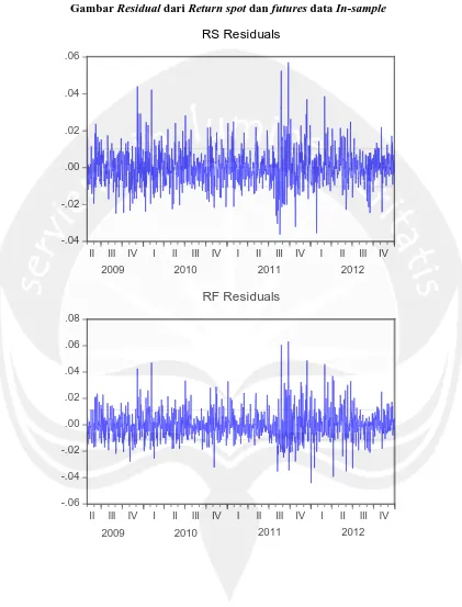
Gambar Residual dari Return spot dan futures data In-sample

-.04 -.02 .00 .02 .04 .06

II III IV I II III IV I II III IV I II III IV

2009 2010 2011 2012

RS Residuals

-.06 -.04 -.02 .00 .02 .04 .06 .08

II III IV I II III IV I II III IV I II III IV

2009 2010 2011 2012

(13)

Estimas Model OLS in-sample

Dependent Variable: RS Method: Least Squares Date: 09/21/13 Time: 18:24 Sample: 5/01/2009 12/31/2012 Included observations: 957

RF 0.212827 0.028068 7.582561 0.0000

(14)

Estimasi penentuan Lag VAR data in-sample

VAR Lag Order Selection Criteria Endogenous variables: RS RF Exogenous variables: C Date: 09/27/13 Time: 10:23 Sample: 5/01/2009 12/31/2012 Included observations: 949

Lag LogL LR FPE AIC SC HQ

0 5930.008 NA 1.29e-08 -12.49317 -12.48293 -12.48927 1 6480.872 1098.245 4.06e-09 -13.64567 -13.61498 -13.63398 2 6563.754 164.8917 3.44e-09 -13.81192 -13.76075 -13.79242 3 6621.806 115.2475 3.07e-09 -13.92583 -13.85420 -13.89854 4 6639.654 35.35674 2.98e-09 -13.95501 -13.86292 -13.91992 5 6658.217 36.69479 2.89e-09 -13.98570 -13.87314* -13.94282 6 6669.072 21.41443 2.85e-09 -14.00015 -13.86713 -13.94947 7 6678.706 18.96234 2.82e-09 -14.01203 -13.85853 -13.95354 8 6691.688 25.49905* 2.76e-09* -14.03095* -13.85700 -13.96467*

* indicates lag order selected by the criterion

LR: sequential modified LR test statistic (each test at 5% level) FPE: Final prediction error

AIC: Akaike information criterion SC: Schwarz information criterion HQ: Hannan-Quinn information criterion Covarian

(15)

Estimasi VAR Models

Vector Autoregression Estimates Date: 09/27/13 Time: 11:07

Sample (adjusted): 5/13/2009 12/31/2012 Included observations: 949 after adjustments Standard errors in ( ) & t-statistics in [ ]

RS RF

RS(-1) -0.782070 0.044175 (0.03818) (0.08202) [-20.4858] [ 0.53858]

RS(-2) -0.655281 -0.071799 (0.04800) (0.10312) [-13.6526] [-0.69625]

RS(-3) -0.507622 -0.086539 (0.05239) (0.11255) [-9.68995] [-0.76887]

RS(-4) -0.432104 0.043394 (0.05303) (0.11394) [-8.14772] [ 0.38084]

RS(-5) -0.318341 0.035080 (0.05232) (0.11241) [-6.08428] [ 0.31206]

RS(-6) -0.219672 0.018097 (0.04754) (0.10214) [-4.62082] [ 0.17718]

RS(-7) -0.137569 0.019868 (0.03941) (0.08468) [-3.49056] [ 0.23464]

RS(-8) -0.023992 0.074387 (0.01840) (0.03952) [-1.30417] [ 1.88205]

RF(-1) 0.885132 -0.045225 (0.01785) (0.03834) [ 49.5973] [-1.17948]

(16)

(0.03844) (0.08259) [ 18.0531] [-0.44351]

RF(-3) 0.624015 0.010826 (0.04596) (0.09874) [ 13.5778] [ 0.10964]

RF(-4) 0.500845 0.061872 (0.05005) (0.10754) [ 10.0063] [ 0.57534]

RF(-5) 0.409071 -0.052761 (0.05093) (0.10943) [ 8.03188] [-0.48216]

RF(-6) 0.297176 -0.054226 (0.04937) (0.10607) [ 6.01975] [-0.51125]

RF(-7) 0.220592 -0.014613 (0.04375) (0.09400) [ 5.04223] [-0.15546]

RF(-8) 0.118568 -0.050586 (0.03380) (0.07262) [ 3.50779] [-0.69657]

C -0.000244 -0.000619

(0.00018) (0.00038) [-1.38944] [-1.64362]

R-squared 0.732083 0.015298 Adj. R-squared 0.727484 -0.001607 Sum sq. resids 0.026414 0.121931 S.E. equation 0.005324 0.011438 F-statistic 159.1682 0.904946 Log likelihood 3630.581 2904.809 Akaike AIC -7.615556 -6.086005 Schwarz SC -7.528578 -5.999027 Mean dependent -0.000579 -0.000562 S.D. dependent 0.010198 0.011429

Determinant resid covariance (dof adj.) 2.67E-09 Determinant resid covariance 2.57E-09

Log likelihood 6691.688

Akaike information criterion -14.03095

(17)

Hasil Variance dan Covariance model VAR

Hasil perhitungan efektivitas Hedging In-sample VAR model

Value

σ

_s

0.000028

σ

_f

0.000131

σ

_sf

0.000032

VarU

0.000028

VarH

0.0000223

HE (

hedging effectiveness

)

0.2559882

Covariance Matrix

RS

RF

RS

0.000028

0.000032

(18)

VEC Model data in-sample

Vector Error Correction Estimates Date: 09/27/13 Time: 11:07

Cointegrating Eq: CointEq1

RS(-1) 1.000000

RF(-1) -0.997292 (0.01024) [-97.3719]

C 2.80E-05

Error Correction: D(RS) D(RF)

CointEq1 -4.131826 0.832749 (0.29402) (0.65167) [-14.0529] [ 1.27786]

D(RS(-1)) 2.349206 -0.760106 (0.27475) (0.60898) [ 8.55020] [-1.24817]

D(RS(-2)) 1.685494 -0.803053 (0.24455) (0.54203) [ 6.89224] [-1.48157]

D(RS(-3)) 1.166911 -0.845213 (0.20787) (0.46073) [ 5.61365] [-1.83450]

D(RS(-4)) 0.723690 -0.731879 (0.16776) (0.37182) [ 4.31394] [-1.96836]

D(RS(-5)) 0.396069 -0.608134 (0.12616) (0.27961) [ 3.13954] [-2.17490]

(19)

(0.08465) (0.18763) [ 1.84416] [-2.65466]

D(RS(-7)) -0.000799 -0.365192 (0.04782) (0.10598) [-0.01670] [-3.44582]

D(RS(-8)) -0.044521 -0.148588 (0.01791) (0.03970) [-2.48565] [-3.74285]

D(RF(-1)) -3.209251 -0.125804 (0.28779) (0.63786) [-11.1515] [-0.19723]

D(RF(-2)) -2.482823 -0.081629 (0.26631) (0.59026) [-9.32310] [-0.13829]

D(RF(-3)) -1.820134 0.005496 (0.23545) (0.52186) [-7.73040] [ 0.01053]

D(RF(-4)) -1.277277 0.131578 (0.19831) (0.43954) [-6.44091] [ 0.29936]

D(RF(-5)) -0.828789 0.116929 (0.15778) (0.34971) [-5.25276] [ 0.33436]

D(RF(-6)) -0.487776 0.088434 (0.11502) (0.25494) [-4.24065] [ 0.34688]

D(RF(-7)) -0.215167 0.092226 (0.07274) (0.16122) [-2.95818] [ 0.57207]

D(RF(-8)) -0.048560 0.029006 (0.03472) (0.07695) [-1.39871] [ 0.37695]

C 5.70E-05 1.24E-05

(20)

R-squared 0.859458 0.479414 Adj. R-squared 0.856889 0.469898 Sum sq. resids 0.027169 0.133469 S.E. equation 0.005405 0.011980 F-statistic 334.5443 50.37937 Log likelihood 3612.905 2858.391 Akaike AIC -7.584188 -5.992385 Schwarz SC -7.492017 -5.900214 Mean dependent 7.82E-06 -1.02E-05 S.D. dependent 0.014288 0.016454

Schwarz criterion -13.74040

Hasil Variance dan Covariance VECM

Covariance Matrix

RS

RF

RS

0.000029

0.000036

RF

0.000036

0.000144

Hasil perhitungan efektivitas Hedging In-sample VEC model

Value

σ

_s

0.000031

σ

_f

0.000144

σ

_sf

0.000036

VarU

0.000029

VarH

0.000022

(21)

Multivariate GARCH data in sample

System: UNTITLED

Estimation Method: ARCH Maximum Likelihood (Marquardt) Covariance specification: Diagonal VECH

Date: 09/27/13 Time: 11:53 Sample: 5/01/2009 12/31/2012 Included observations: 957

Total system (balanced) observations 1914 Presample covariance: backcast (parameter =0.7) Convergence achieved after 11 iterations

Coefficient Std. Error z-Statistic Prob. C(1) -0.000549 0.000312 -1.761110 0.0782 C(2) -0.000584 0.000335 -1.744653 0.0810

Variance Equation Coefficients

C(3) 3.14E-06 1.11E-06 2.834149 0.0046 C(4) 2.52E-06 3.57E-06 0.706725 0.4797 C(5) 2.34E-06 6.82E-07 3.428896 0.0006 C(6) 0.045874 0.008810 5.207112 0.0000 C(7) 0.012196 0.013010 0.937441 0.3485 C(8) 0.039958 0.006278 6.364434 0.0000 C(9) 0.922521 0.016617 55.51771 0.0000 C(10) 0.883863 0.149515 5.911530 0.0000 C(11) 0.941993 0.008381 112.3991 0.0000 Log likelihood 6064.850 Schwarz criterion -12.59582 Avg. log likelihood 3.168678 Hannan-Quinn criter. -12.63043 Akaike info criterion -12.65172

Equation: RS = C(1)

R-squared -0.000021 Mean dependent var -0.000595 Adjusted R-squared -0.000021 S.D. dependent var 0.010183 S.E. of regression 0.010184 Sum squared resid 0.099141 Durbin-Watson stat 1.959502

Equation: RF = C(2)

R-squared -0.000001 Mean dependent var -0.000595 Adjusted R-squared -0.000001 S.D. dependent var 0.011400 S.E. of regression 0.011400 Sum squared resid 0.124252 Durbin-Watson stat 2.070180

Covariance specification: Diagonal VECH

GARCH = M + A1.*RESID(-1)*RESID(-1)' + B1.*GARCH(-1) M is an indefinite matrix

A1 is an indefinite matrix B1 is an indefinite matrix

Transformed Variance Coefficients

(22)

M(1,1) 3.14E-06 1.11E-06 2.834149 0.0046 M(1,2) 2.52E-06 3.57E-06 0.706725 0.4797 M(2,2) 2.34E-06 6.82E-07 3.428896 0.0006 A1(1,1) 0.045874 0.008810 5.207112 0.0000 A1(1,2) 0.012196 0.013010 0.937441 0.3485 A1(2,2) 0.039958 0.006278 6.364434 0.0000 B1(1,1) 0.922521 0.016617 55.51771 0.0000 B1(1,2) 0.883863 0.149515 5.911530 0.0000 B1(2,2) 0.941993 0.008381 112.3991 0.0000

Hasil Variance dan Covariance model M-GARCH

Covariance Matrix

RS

RF

RS

0.000130

0.000027

RF

0.000027

0.000104

Hasil perhitungan efektivitas Hedging In-sample M-GARCH model

Value

h

sst

0.000130

h

fft

0.000104

h

sft

0.000027

VarU

0.000130

VarH

0.000090

(23)

Colegram MGARCH

(24)

.0000 .0001 .0002 .0003 .0004

II III IV I II III IV I II III IV I II III IV

2009 2010 2011 2012

Var(RS)

.00001 .00002 .00003 .00004 .00005 .00006

2009 2010 2011 2012

Cov(RS,RF)

.0000 .0001 .0002 .0003 .0004 .0005

2009 2010 2011 2012

Var(RF)

(25)

LAMPIRAN 2

Perhitungan Out of sample

ADF Return Spot out of sample

Null Hypothesis: RS3 has a unit root Exogenous: Constant

t-Statistic Prob.*

5% level -2.910019

10% level -2.592645

Augmented Dickey-Fuller Test Equation Dependent Variable: D(RS3)

RS3(-1) -1.119179 0.130169 -8.597878 0.0000 C 0.000922 0.000973 0.947258 0.3474

(26)

ADF Futures Return out of sample

Null Hypothesis: RF3 has a unit root Exogenous: Constant

t-Statistic Prob.*

5% level -2.910019

10% level -2.592645

Augmented Dickey-Fuller Test Equation Dependent Variable: D(RF3)

RF3(-1) -1.021681 0.129462 -7.891777 0.0000 C 0.000962 0.000929 1.036124 0.3044

(27)

Model OLS out of sample

Dependent Variable: RS3 Method: Least Squares Date: 10/06/13 Time: 12:33 Sample: 1/02/2013 3/28/2013 Included observations: 62

RF3 0.314839 0.127099 2.477127 0.0160

(28)

Estimasi Lag VAR out of sample

VAR Lag Order Selection Criteria Endogenous variables: RS3 RF3 Exogenous variables: C

Lag LogL LR FPE AIC SC

0 412.5278 NA 1.90e-09 -14.40448 -14.33280 1 443.6076 58.88810 7.36e-10 -15.35465 -15.13960 2 458.4569 27.09338 5.03e-10 -15.73533 -15.37690* 3 461.3524 5.079959 5.24e-10 -15.69658 -15.19478 4 466.4217 8.537667 5.06e-10 -15.73409 -15.08892 5 478.5704 19.60843* 3.82e-10* -16.02001* -15.23147

* indicates lag order selected by the criterion

LR: sequential modified LR test statistic (each test at 5% level) FPE: Final prediction error

(29)

VAR Model

Vector Autoregression Estimates Date: 10/06/13 Time: 12:36

RS3 RF3

RS3(-1) -0.662796 0.613198 (0.15573) (0.29079) [-4.25612] [ 2.10874]

RS3(-2) -0.911549 -0.390183 (0.19390) (0.36206) [-4.70119] [-1.07767]

RS3(-3) -0.608593 -0.358521 (0.19583) (0.36567) [-3.10778] [-0.98045]

RS3(-4) -0.604321 -0.918408 (0.16361) (0.30550) [-3.69377] [-3.00626]

RS3(-5) -0.154452 -0.077537 (0.08924) (0.16663) [-1.73080] [-0.46532]

RF3(-1) 1.008030 -0.039523 (0.08919) (0.16654) [ 11.3020] [-0.23731]

RF3(-2) 0.677413 -0.345946 (0.17351) (0.32400) [ 3.90411] [-1.06774]

RF3(-3) 0.703686 0.602968 (0.19758) (0.36894) [ 3.56152] [ 1.63433]

RF3(-4) 0.556757 0.469040 (0.16888) (0.31535) [ 3.29679] [ 1.48738]

(30)

(0.11564) (0.21593) [ 4.34209] [ 2.90895]

C 0.000356 0.000499

(0.00044) (0.00081) [ 0.81552] [ 0.61327]

R-squared 0.791376 0.396291 Adj. R-squared 0.746023 0.265050 Sum sq. resids 0.000466 0.001625 S.E. equation 0.003183 0.005943 F-statistic 17.44926 3.019566 Log likelihood 252.9847 217.3889 Akaike AIC -8.490692 -7.241718 Schwarz SC -8.096419 -6.847444 Mean dependent 0.000572 0.000736 S.D. dependent 0.006315 0.006932

Hasil Variance dan Covariance model VAR

Covariance Matrix

RS3

RF3

RS3

0.000010

0.000009

RF3

0.000009

0.000035

Hasil perhitungan efektivitas Hedging out of sample VAR model

Value

σ

s

0.000010

σ

f

0.000035

σ

sf

0.000009

VarU

0.000010

VarH

0.000004

(31)

VECM

Vector Error Correction Estimates Date: 10/06/13 Time: 12:37

Cointegrating Eq: CointEq1

RS3(-1) 1.000000

RF3(-1) -0.937808 (0.03549) [-26.4241]

C -0.000127

Error Correction: D(RS3) D(RF3)

CointEq1 -3.589420 0.901328 (0.90591) (1.78743) [-3.96221] [ 0.50426]

D(RS3(-1)) 1.940068 -0.098188 (0.79747) (1.57346) [ 2.43278] [-0.06240]

D(RS3(-2)) 0.963868 -0.311185 (0.65229) (1.28701) [ 1.47767] [-0.24179]

D(RS3(-3)) 0.529345 -0.136957 (0.44588) (0.87976) [ 1.18718] [-0.15568]

D(RS3(-4)) 0.034017 -0.586025 (0.25326) (0.49969) [ 0.13432] [-1.17277]

D(RS3(-5)) 0.012800 -0.096622 (0.08917) (0.17594) [ 0.14355] [-0.54919]

(32)

D(RF3(-2)) -1.590170 -0.466053 (0.68352) (1.34864) [-2.32643] [-0.34557]

D(RF3(-3)) -0.829833 0.000786 (0.51720) (1.02048) [-1.60446] [ 0.00077]

D(RF3(-4)) -0.397938 0.028210 (0.31310) (0.61777) [-1.27096] [ 0.04566]

D(RF3(-5)) 0.041286 0.352718 (0.14267) (0.28151) [ 0.28937] [ 1.25297]

C -0.000172 0.000110

(0.00044) (0.00087) [-0.38839] [ 0.12559]

R-squared 0.890044 0.673464 Adj. R-squared 0.862555 0.591831 Sum sq. resids 0.000462 0.001797 S.E. equation 0.003239 0.006390 F-statistic 32.37808 8.249814 Log likelihood 248.3174 210.2603 Akaike AIC -8.439906 -7.080724 Schwarz SC -8.005902 -6.646720 Mean dependent -2.35E-05 5.70E-05 S.D. dependent 0.008736 0.010002

Hasil Variance dan Covariance VECM

Covariance Matrix

RS3

RF3

RS3

0.000010

0.000011

(33)

Hasil perhitungan efektivitas Hedging out of sample VEC model

Value

σ

s

0.000010

σ

f

0.000041

σ

sf

0.000011

VarU

0.000010

VarH

0.000005

(34)

M-GARCH MODEL

System: UNTITLED

Estimation Method: ARCH Maximum Likelihood (Marquardt) Covariance specification: Diagonal VECH

Total system (balanced) observations 124 Presample covariance: backcast (parameter =0.7) Convergence achieved after 61 iterations

Coefficient Std. Error z-Statistic Prob. C(1) 0.000605 0.001160 0.521412 0.6021 C(2) 0.000605 0.001093 0.553183 0.5801

Variance Equation Coefficients

C(3) 1.05E-05 1.08E-05 0.970466 0.3318 C(4) 6.71E-06 1.22E-05 0.547631 0.5839 C(5) 4.45E-05 4.35E-05 1.024539 0.3056 C(6) -0.003396 0.074767 -0.045420 0.9638 C(7) -0.107410 0.187037 -0.574272 0.5658 C(8) 0.226009 0.298664 0.756733 0.4492 C(9) 0.751773 0.224056 3.355296 0.0008 C(10) 0.692759 0.638183 1.085517 0.2777 C(11) -0.072382 0.826461 -0.087581 0.9302 Log likelihood 444.2450 Schwarz criterion -13.59825 Avg. log likelihood 3.582621 Hannan-Quinn criter. -13.82747 Akaike info criterion -13.97565

Equation: SS = C(1)

R-squared -0.000379 Mean dependent var 0.000750 Adjusted R-squared -0.000379 S.D. dependent var 0.007493 S.E. of regression 0.007495 Sum squared resid 0.003427 Durbin-Watson stat 2.209511

Equation: FF = C(2)

R-squared -0.000807 Mean dependent var 0.000807 Adjusted R-squared -0.000807 S.D. dependent var 0.007186 S.E. of regression 0.007189 Sum squared resid 0.003153 Durbin-Watson stat 2.005836

Covariance specification: Diagonal VECH

GARCH = M + A1.*RESID(-1)*RESID(-1)' + B1.*GARCH(-1) M is an indefinite matrix

A1 is an indefinite matrix* B1 is an indefinite matrix*

Transformed Variance Coefficients

(35)

M(1,1) 1.05E-05 1.08E-05 0.970466 0.3318 M(1,2) 6.71E-06 1.22E-05 0.547631 0.5839 M(2,2) 4.45E-05 4.35E-05 1.024539 0.3056 A1(1,1) -0.003396 0.074767 -0.045420 0.9638 A1(1,2) -0.107410 0.187037 -0.574272 0.5658 A1(2,2) 0.226009 0.298664 0.756733 0.4492 B1(1,1) 0.751773 0.224056 3.355296 0.0008 B1(1,2) 0.692759 0.638183 1.085517 0.2777 B1(2,2) -0.072382 0.826461 -0.087581 0.9302 * Coefficient matrix is not PSD.

Hasil Variance dan Covariance model M-GARCH

Covariance Matrix

RSM

RFM

RSM

0.000055

0.000016

RFM

0.000016

0.000051

Hasil perhitungan efektivitas Hedging Out of sample M-GARCH model

Value

h

sst

0.000055

h

fft

0.000051

h

sft

0.000016

VarU

0.000055

VarH

0.000006