GEO-ENVIRONMENTAL APPRAISAL FOR STUDYING URBAN ENVIRONMENT AND
ITS ASSOCIATED BIOPHYSICAL PARAMETERS USING
REMOTE SENSING AND GIS TECHNIQUE
Kuntal Ganguly a, *, G. Ravi Shankar a a
National Remote Sensing Centre, ISRO, DOS, Hyderabad – [email protected], [email protected]
KEY WORDS: Urban Environment, SAVI, MNDWI, IBI, LST, IRS Resourcesat-2 LISS-3, Landsat TM/ETM+/8, CORONA
ABSTRACT:
This study investigated the influences of urbanization on urban ecological and thermal environment as well as the relationships of all the biophysical parameters with each other utilizing multi-temporal datasets of CORONA (1967), Landsat TM (1992 and 2009), Landsat ETM+ (2002), IRS R2 LISS-3 (2012) and Landsat 8 (2014). The urban environmental issues related to land use and land cover, greenness, surface wetness and impervious surface were assessed using change detection, SAVI, MNDWI and IBI models respectively. The land surface temperature (LST) was also retrieved from thermal infrared band of each Landsat TM, ETM+ and Landsat 8. Based on these parameters, the urban expansion, urban heat island effect and the relationships of LSTs to other biophysical parameters were analyzed. Results indicate the area ratio of impervious surface in Pune sub-urban zone increased significantly, which grew from 1.41% in 1967 to 8.47% in 1992 and further to 22.45% and 44.7% in 2002 and 2014 respectively. Simultaneously, the intensity of urban heat island increased in observed years. A correlation analyses revealed that, the association of impervious surface to other two variables i.e. greenness and land surface wetness is negatively correlated (R2 = 0.616 and 0.607 respectively). Whereas, LST possessed a strong positive correlation with impervious surfaces (R2 = 0.658).
The present study provided an integrated research approach and the outcome of the study is very useful in environmental modelling and sustainable development of urban areas and natural resources conservation.
*Corresponding author at: National Remote Sensing Centre, ISRO, DOS, Balanagar, Hyderabad 500037, India Phn: +91 7303916539
E-mail address: [email protected] (K. Ganguly)
1. INTRODUCTION
There is an unequal urban growth, which is taking place all over the world, but the rate of urbanization is very fast in the developing countries, especially in Asia. In 1800 A.D., only 3% of the world’s population lived in urban centres, but this figure reached to 14% in 1900 and in 2000, about 47% (2.8 billion) people were living in urban areas. India no longer lives in villages and 79 million people were living in urban areas in 1961, but it went up to 285 million in 2001. In India and China alone, there are more than 170 urban areas with populations of over 750,000 inhabitants (United Nations Population Division, 2001). Statistics show that India’s urban population is the second largest in the world after China, and is higher than the total urban population of all countries put together barring China, USA and Russia. In 1991, there were 23 metropolitan cities in India, which increased to 35 in 2001 (Census of India, 1991 and 2001).
With rapid urbanization, there has been a tremendous growth in population and buildings in cities, which lead to the drastic reduction in the greenery area and oppositely the increase in impervious area. The core of the city becomes warmer than its periphery, thus forming an Urban Heat Island-UHI (Voogt and Oke, 2003). Over the past few years, remotely sensed data of various spatial, spectral, angular, and temporal resolutions have been widely used to study the land use and land cover
changes associated with urban growth, and to retrieve land surface biophysical parameters, such as vegetation abundances, built-up indices and land surface temperatures, that are good indicators of conditions of urban ecosystem (Streutker, 2002; Sobrino et al., 2004; Xu, 2008a,b; Luand Weng, 2009; Tooke et al., 2009; Zhang et al., 2009).
Geo-environmental appraisal deals with every issue that affects a living organism in the world. It is essentially a multidisciplinary approach that brings about an appreciation of our natural world and human impact on its integrity. One of such approaches is to prepare regional geo-environmental appraisal for identification of areas subject to environmental degradation.
The galloping process of industrialization, urbanization and globalization has brought mounting environmental problems including climate change, water shortage and pollution, hazardous waste, smog, loss of bio-diversity and desertification that pose severe challenges to sustainable development. Environmental considerations are assuming greater importance in the urban planning processes of an increasing number of governments around the world. Pune city, now home to more than 3.1 million population, is growing at a rapid pace, increasingly at the forefront of the most pressing environmental challenges which require government, public and private organizations and individuals to take a fresh
perspective at how economic and social activities can best be organized in the existing urban environment.
Greenness or vegetation abundance to study eco-environment plays a crucial role in the exchange of material and energy over land surface. Accurate mapping and monitoring of spatio-temporal dynamics of vegetation in urban area is essential to understand urban ecosystems, including its role in mitigating air pollution and reducing the urban heat island effect (Small and Lu, 2006), however, the accuracy could hardly meet the current application requirement due to the existence of mixture pixels, especially in urban area.
Impervious land surface, as one of the most important land cover types and characteristics of urban/suburban environments, is known to affect urban surface temperatures. However, this may not produce satisfactory accuracy due to the high incidence of mixture pixel in urban area (Xu, 2008b). To analyze the UHI effect in study area, LSTs were also retrieved from TM/ETM+ TIR bands.
Near surface soil moisture (SM), defined as the water content of the upper 10 cm of the soil (Wang and Qu, 2009), is measured by remote sensing satellites using the electromagnetic radiation in three distinct ranges: the visible and near-infrared region, thermal region and the microwave region. Image analysis and interpretation techniques such as soil wetness indexes, directly (Bhagat, 2009) or indirectly (Sørensen et al., 2005, Grabs et al., 2009) using remotely sensed data in the visible and near-infrared region are applied to estimate wetness of the near-surface soil layer.
The correlations were analysed between land surface temperatures, vegetation abundance and surface wetness with impervious surface. Finally the conclusions and a brief discussion were given in the last section.
2. MATERIALS AND METHOD
2.1 Study area
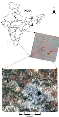
The study area comprises a part of Pimpri Chinchwad Municipal Corporation (PCMC), lies between 73o 41’ 16” E to 73o 52’ 22” E and 18o 34’ 58” N to 18o 43’ 22” N, was an underdeveloped village, surrounded by Pavana, Mula and Mutha river. The geomorphological setting of the city side shows a backdrop of hills on the south and south western sides, with steeper slopes and rocky red soils. The area is underlain by basaltic lava flows of upper cretaceous econe age associated with basic intrusive. The soil texture contains alluvial deposits of sand, gravels, fine silts and clays along the bank of the rivers. Prior to its development, most of the inhabitants were poor peasants practicing agriculture and wood carving, deprived of basic public services.
The area came under PCMC in 1982 and from the late 1990s the village grew to catch up with the vast industrialization and expansion of Pune city. Thereafter the approval of PCMC for vast industrialization and construction has pushed up air and noise pollution levels here and industrial waste being flushed into its water bodies has added to their filth, with Pavana River emerging as the most polluted of the three rivers flowing here. Unabated growth in this sub urban zone of Pune city has resulted in depletion of natural resources affecting the quality of life.
Figure 1. Location of the study area
2.2 Data used
Landsat TM images of February 04, 1992 and March 22, 2009, Landsat ETM+ image of March 27, 2002, Landsat 8 image of April 04, 2014, IRS Resourcesat-2 LISS-3 of March 17, 2012 and a CORONA image of November 11, 1967 were used in this study, acquired under clear sky conditions. Except CORONA image, all other images were geometrically corrected and georeferenced to the WGS-84 datum and Universal Transverse Mercator zone 43N coordinate system. The declassified CORONA image was corrected geometrically with a RMS error 0.238. The detail of the satellite images is given below.
Table 1. Satellite image specifications
2.3 Software used
In the present study datasets were analysed using ArcGIS 10.2.1 and Erdas imagine 2014 for deriving spatial information and indices. Microsoft excel 2007 has been used for statistical analysis.
Sensor
Mode Sensor Platform Date
Path/ Row
MS
TM
ETM+
Landsat 8
R2-LISS 3
Landsat 5
Landsat 7
Landsat 8
IRS
04-02-1992
22-03-2009
27-03-2002
05-04-2014
17-03-2012
147/47
PAN Corona J3 CORONA 11-11-1967
MNDWI = GREEN−MIR dominant land-cover classes in the study area, unsupervised classification method was used. Iterative classification process was carried out using Landsat TM/ETM+/Landsat-8 and IRS R2 LISS-3 image acquired over the study area. Five dominant land cover classes were extracted in the region. With the order of highest to the lowest percentage these classes included built-up, water bodies, crop land/fallow, scrub/waste land, vegetation. The in-situ sites were chosen only on five LC classes due to the issues in finding suitable sites for some of the land cover types.
2.4.2 Surface wetness estimation: Water area accounts for a small percentage in our study area, however, vegetation abundance and impervious surface posses nearly zero values in these areas, thus it was advisable to include surface wetness negative values signify dry area.
2.4.3 Estimation of greenness: The heat island phenomenon is occurring in urban areas where heat builds up through the artificial ground surface cover, the increase in artificial waste heat, and the extreme advancement of the destruction of natural environment. Incorporating a greenness index, site specific information can be achieved. In the present study soil adjusted vegetation index (SAVI) was used to measure the temporal variation of surface greenness with the advancement of the sub-urban zone. This index is similar to NDVI, but it suppresses the effects of soil pixels. It uses a canopy background adjustment factor, L, which is a function of vegetation density and often requires prior knowledge of vegetation amounts. Huete (1988) suggests an optimal value of L= 0.5 to account for first-order soil background variations. This index is best used in areas with relatively sparse vegetation where soil is visible through the canopy.
(2)
Eq. (2) produces values in the range from -1 to +1 where positive values indicate greenness or wet area and negative values signify less vegetation.
2.4.4 Derivation of impervious surface: Impervious surface is one of the most important land cover types and also a key indicator of urban expansion and urban heat island effect. To effectively map the dynamics of the impervious surface an integrated built up extraction approach was taken place. Extraction and classification of settlement areas were quickly done based on approach to Index-based Built-up Index (IBI), as was done by Xu (2007). The development of the Index-based Built-up Index (IBI) approach in the study was done by adding multiple indices, which was expressed by:
(3)
(4)
Where, NDBI is the normalized difference vegetation index (Eq. (3)); MIR and NIR are the digital numbers of near and middle infrared band MNDWI is modified normalized difference water index (Eq. (1)) and SAVI is soil adjusted vegetation index (Eq. (2)). Derived IBI was used to extract impervious surface by classification of settlement areas and non-settlement area.
2.4.5 Estimation of land surface temperature: Studies have been done on the relative warmth or “heat island effect” of cities by measuring the air temperature, using meteorological data. However, this method is time consuming and it leads to problems in spatial interpolation. Hence satellite sensors can provide quantitative physical data at high spatial and temporal resolutions and repetitive coverage is capable of measurements of earth surface conditions overtime (Owen et al., 1998). A variety of algorithms have been developed to retrieve land surface temperature from TM/ETM+ imagery, such as mono-window algorithm (Qin et al., 2001), single-channel algorithm (Jimenez-Munoz and Sobrino, 2003) and the method proposed by Artis and Carnahan (1982). In the present study several image transformation techniques were used to retrieve the land surface temperature (LST). The following equation was used to convert the digital number (DN) of Landsat5- TM TIR band to spectral radiance (Markham and Barker, 1985):
Lλ= 0.05518*DN+1.2378 (5)
For Landsat-7 ETM+ band 6 is captured twice: once in low-gain (e.g. Landsat-8 band 10) and the other in high-low-gain mode (e.g. Landsat-8 band 11). Low-gain mode is used to image
Landsat TM Landsat ETM+ Landsat 8
K1 607.76 666.09 774.89
For Landsat 8 can be expressed by:
Lλ = ML * QCAL + AL (7)
Where ML is the band specific multiplicative rescalling factor from the metadata ( RADIANCE_MULT_BAND_DN), AL is the band specific additive rescaling factor from the metadata (RADIANCE_ADD_BAND_DN), QCAL is the quantized and
T = K2 ln ( K1
Lλ + 1)
calibrated standard product pixel values (DN) (USGS Landsat 8 product, 2013).
Then the following formula was used to convert the spectral radiance to at-sensor brightness temperature under the assumption of uniform emissivity (Landsat Project Science Office, 2002; Wukelic et al., 1989):
(8)
Where, T is at-satellite brightness temperature (K), Lλ is TOA spectral radiance (Watts/ (m2*srad*µm)), K2 and K1 are the prelaunch calibration constants, which are listed in Table 2. Then the following formula was used to convert the temperature in degree Kelvin to degree Celsius.
C = T – 273 (9)
Where, C is the brightness temperature in degree Celsius, T is degrees in Kelvin and Kelvin is 273 degrees lower than Celsius.
3. RESULTS AND DISCUSSION
3.1 Land use and land cover dynamics
Comparison of the land use and land cover maps revealed significant changes occurred since last 47 years (1967 to 2014). Greatest change has been observed on the built-up site, while the other LC types have relatively similar trends of over the 47 years period. Crop land and scrubland has reduced remarkably and the surface moisture condition also reduced. Land use/land cover maps were produced from multi-spectral satellite images. The CORONA scan photo also used for past reconstruction of land use but still the digital classification on CORONA had some limitations. The sub-class level land use statistics from CORONA data was ignored for analysis. The study shows that out of study area’s total area of 32012 ha, agriculture constituted 18435.69 ha in 1992, and this declined by 12.5% to 14436.04 ha. by 2002. There was a reduction of 20.18% to 7975.09 ha. by 2014. The major cause of this unprecedented decline in area under agriculture was due to an increase in urban area (Table 3 and Figure 2). At the same time high density residential area more than doubled in the last twelve years, mainly at the cost of fertile agricultural land. Similarly land transformations have taken place all around Pune city in the fringe areas especially in western part of Pune. High density industrial and residential areas have replaced low and medium density industrial and residential areas. There was a considerable decrease in the vegetative area, from 4.87% in 1992 to 3.59% in 2014, because of continuous illegal tree cutting and construction activity.
Accuracy assessment of all the land use and land cover classes has been done using ground truth data and ArcGIS 10.2.1 spatial analyst tool. Confusion matrix generated for all datasets revealed an overall 98 % accuracy for built-up, crop land and waste land, where as overall 85% and 78% accuracy was achieved for water bodies and vegetation respectively.
Area (in ha.) 1967 1992 2002 2014
Built-up 452.12 2711.60 7186.86 14310.46
Crop land /
Fallow land 18548.76 18435.69 14436.04 7975.09
Vegetation 137.34 1560.33 1468.02 1149.17
Scrub land /
Waste land 12425.43 8767.26 8467.26 8127.28 Water bodies 448.35 537.12 453.83 450.00
Figure 3. Land use and land cover change dynamics (a) (b)
3.2 Impervious surface dynamics
A variety of enhancement techniques have been used to extract the built up area from multi-spectral satellite images under section 2.4.4. A comparison analysis was consequently employed between NDBI and IBI to investigate the performance of these methods, and then to determine which method was suitable for accurately and easily enhancing the impervious surface of the study area. Bare soil has a higher reflectance and as 25% of the study area was dominated by bare soil thus IBI had a biased result in some portions of the study area. To eliminate the error an unsupervised classification was introduced to extract the impervious surface and others were classified as non-built-up areas (Figure 4).
Figure 4. Impervious surface of the study area in 1967 (a), 1992 (b), 2002 (c) and 2014 (d)
Table 3 shows that sub-urban zone of Pune city, currently a part of Pune Chinchwad Municipal Corporation, experienced a rapid urbanization from 1967 to 2014, which was witnessed by the significant enlargement of area ratio of impervious surface in study area, i.e. it grew from 1.41% in 1967 to 8.47% in 1992, and further to 22.45% and 44.70% in 2002 and 2014. The result shows the rate of increase of impervious surface area mainly occurred near the north-western part of the Pune city and in between Mula and Mutha River between 1992 and 2014. Now this rapid expansion of built-up area of the sub-urban zone significantly influences the eco-environment and the people are experiencing threat to protect the urban eco-environment.
3.3 Spatio-temporal dynamics of land surface temperature
To estimate the surface temperature, derivation of surface emissivity is important. Since the study area is a heterogeneous one, estimation of surface emissivity at the pixel scale was calculated. In the present study surface temperature was estimated and mapped using Landsat TM of 1992 and 2009, ETM+ of 2002 and Landsat-8 thermal channel of 2014. Table 4 shows that there is a gradual increase of surface temperature. It was observed that in the image, the central and eastern parts exhibit a maximum surface
temperature range that corresponds to built-up areas, wastelands, bare soil, and fallow lands (Figure 5).
Table 4. Variations in temperature for observed years
The intensities of LST for four dates were listed in Table 4. Results indicated that there was an ongoing expansion of built-up areas and simultaneous raise of temperature in observed years. The maximum surface temperature increased from 33.18o C of 1992 to 39.56o C of 2014, although decrease in minimum temperature was recorded to 17.63o C during 2009.
Figure 5. Land surface temperature dynamics of the study area in 1967 (a), 1992 (b), 2002 (c) and 2014 (d)
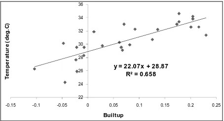
Correlation studies have been made to assess the relationship between surface temperature and impervious surface from 1992 to 2014. Results indicate a significant and positive correlation (R2 = 0.658) between above mentioned parameters (Figure 6), which reflects 65.8 percent of the variations in LST was due to presence of impervious surface.
y = 22.07x + 28.87 R² = 0.658
22 24 26 28 30 32 34 36
-0.15 -0.1 -0.05 0 0.05 0.1 0.15 0.2 0.25
T
e
m
p
e
r
a
tu
r
e
(
d
e
g
. C
)
Builtup
Figure 6. Relationship of LST to impervious surface Temperature (Degree Celsius)
Year Max Min
1992 33.18 15.93
2002 35.36 18.26
2009 39.5 17.63
2014 39.56 22.35
(a) (b)
(c) (d)
(a) (b)
(c) (d)
3.4 Land surface greenness and urban expansion
Visually, the synthetic images generated by SAVI model, distinguish the vegetated and non-vegetated areas. Though the sparse vegetation characteristic gives bias SAVI result, but still a trend of gradual decrease of greenness was observed in SAVI images from 1992 to 2014 (Table 5).
SAVI Ranges
Year Max Min
1992 0.92 -1.00
2002 0.46 -0.20
2009 0.31 -0.07
2014 0.20 -0.15
Table 5. Variations in vegetation cover for observed years
Results showed a very high SAVI value (0.92) in 1992, whereas a 50% reduction of greenness (0.46) was observed in 2002 and thereafter a gradual decrease of SAVI sets very low (0.2) vegetation cover in the study area in 2014 (Figure 7).
Figure 7. SAVI derived from Landsat TM (a and c), ETM+ (b) and Landsat 8 (d) imagery for four different dates
Figure 8. Histogram showing distribution of greenness in 1992 (a), 2002 (b), 2009 (c) and 2014 (d)
The histogram also showed the same trend as the SAVI is very high in 1992 and approaching towards positive, whereas the distribution tends to negative from 2002 to 2014 (Figure 8).
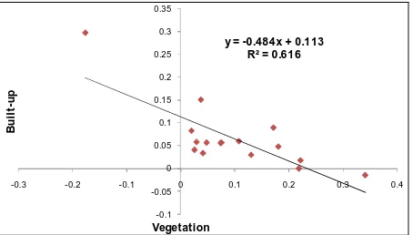
The graph of 2014 showed a normal distribution, which indicates a very low vegetated area. Correlation has been made to assess the relationship between greenness and impervious surface. Results indicate both the parameters are negatively correlated (R2 = 0.616) between above mentioned parameters (Figure 9), which reflects 61.6 percent of the variation in vegetations was due to presence of impervious surface.
y = -0.484x + 0.113 R² = 0.616
-0.1 -0.05 0 0.05 0.1 0.15 0.2 0.25 0.3 0.35
-0.3 -0.2 -0.1 0 0.1 0.2 0.3 0.4
B
u
il
t-u
p
Vegetation
Figure 9. Relationship between built-up area and vegetation
3.5 Land surface wetness and urban expansion
In the present study like all other bio-physical parameters, the surface wetness of the study area was assessed to find out the relationship with urban expansion. Land use classes in Table 3 showed only 1.4 percent of the study area under water body class. Although a very little change was observed in surface wetness, but still an assessment has been made using MNDWI model to distinguish wet and dry area. Results showed a high wetness condition during 1992 and 2002, whereas, a gradual decrease of wetness has been observed up to 2014 (Table 6 and Figure 10).
MNDWI Ranges
Year Max Min
1992 0.85 -0.72
2002 0.79 -0.74
2009 0.59 -0.9
2014 0.59 -0.37
Table 6. Variations in surface wetness for observed years
Figure 10. MNDWI showing the dynamics of surface wetness in 1992 (a), 2002 (b), 2009 (c) and 2014 (d) (a) (b)
(c) (d)
(a) (b)
(c) (d)
(a) (b)
(a) (b)
Histogram also showed a negative distribution from 1992 to 2009, whereas in 2014 the graph showed a normal distribution which indicates without moisture or very low surface moisture (Figure 11).
Figure 11. Histogram showing distribution of surface wetness in 1992 (a), 2002 (b), 2009 (c) and 2014 (d)
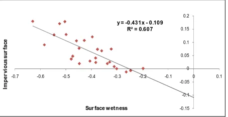
Results of correlation studies between wetness and built-up indicate negative correlation (R2 = 0.607) (Figure 12), which indicates 60.7 percent of the variation in surface wetness was due to presence of impervious surface.
y = -0.431x - 0.109
Figure 12. Relationship between surface wetness and impervious surface
4. CONCLUSIONS
In this paper, multi-temporal Landsat TM/ETM+/Landsat8 and IRS R2 LISS-3 imagery of 1992, 2002, 2009 and 2014 were used to investigate the influences of urbanization on it biophysical variables in sub-urban zone of Pune city. A new integrated method employed to extract the built-up lands was developed. To extract the impervious surface new integrated enhancement method was demonstrated. The urbanization analyses showed that study area or part of PCMC experienced a rapid urbanization since 1992, i.e. the area ratio of impervious surface grew from 1.41% in 1967, to 8.47% in 1992, and further to 22.45% and 44.7% in 2002 and 2014 respectively. Opposite trends of Urban Heat Island intensity before and after 2002 were observed in this study, which implied that not enough attention was taken to the environmental protection in the early stage of urbanization. Comparative analyses of the relationships of LSTs to other variables indicated that at the pixel-scale, the relationships of LSTs to greenness and impervious surfaces were relatively
more complicated due to the variations of the LSTs. However, LSTs possessed a strong positive correlation with percent impervious surfaces and negative correlation with vegetation at the regional-scale, respectively and the correlation coefficients were more than 0.60 for any dataset.
ACKNOWLEDGEMENTS
Authors places on record their deep sense of gratitude to Dr. V.K. Dadhwal, Director, NRSC and Dr. P.G. Diwakar, Deputy Director, NRSC, Hyderabad for their support and motivation to do the work. The authors are also grateful to Dr. T. Ravishankar, Head, LRUMG, NRSC, Hyderabad for his support. The authors thankfully acknowledge the support extended by Shri Rajiv Kumar and Dr. Manoj Raj Saxena, Dr. G. Padmarani, Scientists, NRSC for their support and valuable suggestions to carry out the work.
Authors are also thank to Dr. Tarik Mitran and Mrs. Divya Vijayan, Scientists, NRSC, Hyderabad for their continuous help rendered in this work.
REFERENCES
Artis, D.A. and Carnahan, W.H., 1982. Survey of emissivity variability in thermography of urban areas. Remote Sensing of Environment, 12 (4), pp. 313–329.
Bhagat, V.S., 2009. Use of Landsat ETM+ data for detection of potential areas for afforestation. International Journal of Remote Sensing, 30(10), pp. 2607–2617.
Census of India, 1991 and 2001. Provisional Population Totals, Office of Registrar General of India, Government of India, New Delhi.
Huete, A., 1988. A Soil-Adjusted Vegetation Index (SAVI). Remote Sensing of Environment, 25, pp. 295-309.
Munoz, J.C. and Sobrino, J.A., 2003. A generalized single channel method for retrieving land surface temperature from remote sensing data. Journal of Geophysical Research 108(D22), DOI: 10.1029/2003JD003480.
Landsat Project Science Office, 2002. Landsat 7 Science Data User’s Handbook. Goddard Space Flight Center, NASA, and
Ma, Y., Kuang, Y. and Huang, N., 2010. International Journal of Applied Earth Observation and Geoinformation, 12, pp. 110-118.
Markham, B.L. and Barker, J.K., 1985. Spectral characteristics of the LANDSAT Thematic Mapper sensors. International Journal of Remote Sensing, 6(5), pp. 697–716.
Owen, T.W., Carlson, T.N. and Gillies, R.R., 1998. Remotely Sensed Surface Parameters Governing Urban Climate Change,
(a) (b)
(c) (d)
International Journal of Remote Sensing, 19, pp. 1663-1681.
Qin, Z., Karnieli, A. and Berliner, P., 2001. A mono-window algorithm for retrieving land surface temperature from Landsat TM data and its application to the Israel–Egypt border region. International Journal of Remote Sensing, 22(18), pp. 3719– 3746.
Small, C.J. and Lu, W.T., 2006. Estimation and vicarious validation of urban vegetation abundance by spectral mixture analysis. Remote Sensing of Environment, 100(4), pp. 441– 456.
Sobrino, J.A., Jime´nez-Muoz, J.C. and Paolini, L., 2004. Land surface temperature retrieval from landsat TM5. Remote Sensing of Environment, 90(4), pp. 434–446.
Sørensen, R., Zinko, U. and Seibert, J., 2005. On the calculation of the topographic wetness index: evaluation of different methods based on field observations. Hydrology and Earth System Sciences Discussions, 2(4), pp. 1807–1834.
Streutker, D.R., 2002. A remote sensing study of the urban heat island of Houston, Texas. International Journal of Remote Sensing, 23(13), pp. 2595–2608.
Tooke, T.R., Coops, N.C., Christen, A. and Voogt, J.A., 2009. Extracting urban vegetation characteristics using spectral mixture analysis and decision tree classifications. Remote Sensing of Environment, 113(2), pp. 398–407.
United Nations Population Division, 2001. World Population Prospects: The 2000 Revision, New York.
USGS (United State Geological Survey) landsat 8 product, 2013 USGS. http:// www.landsat.usgs.gov/Landsat8_Using _Product.php.
Voogt, J.A. and Oke, T.R., 2003. Thermal remote sensing of urban climates. Remote Sensing of Environment, 86(3), pp. 370-384.
Wang, L. and Qu, J., 2009. Satellite remote sensing applications for surface soil moisture monitoring: A review. Frontiers of Earth Science in China, 3, pp. 237–247.
Wukelic, G.E., Gibbons, D.E., Martucci, L.M. and Foote, H.P., 1989. Radiometric calibration of Landsat Thematic Mapper thermal band. Remote Sensing of Environment, 28, pp. 339–347.
Xu, H., 2007. A New Index for Delineating Built-up Land Features in Satellite Imagery. International Journal of Remote Sensing, 29(14), pp. 4269-4276.
Xu, H., 2006. Modification of normalized difference water index (NDWI) to enhance open water features in remotely sensed imagery. International Journal of Remote Sensing, 27(14), pp. 3025–3033.
Xu, H., 2008b. A new index for delineating built-up land features in satellite imagery. International Journal of Remote Sensing, 29(14), pp. 4269–4276.
Xu, H.Q., 2008a. A new remote sensing index for fastly extracting impervious surface information. Geomatics and Information Science of Wuhan University, 33, pp. 1150–1153. ISSN. 1671-8860.
Zhang, Y.S., Odeh, Inakwu, O.A. and Han, C.F., 2009. Bi-temporal characterization of land surface temperature in relation to impervious surface area, NDVI and NDBI, using a sub-pixel image analysis. International Journal of Applied Earth Observation and Geoinformation, 11(4), pp. 256–264.