Analysis of Point Cloud Generation from UAS Images
S. Ostrowski, G. Jóźków, C. Toth, B. Vander Jagt
Satellite Positioning and Inertial Navigation (SPIN) Laboratory, The Ohio State University, Department of Civil, Environmental and Geodetic Engineering, 470 Hitchcock Hall, 2070 Neil Avenue, Columbus, OH 43210-1275, (Ostrowski.20, Jozkow.1, Toth.2,
Vander-Jagt.1)@osu.edu
Commission I, WG I/Vb
KEY WORDS: UAS, Point Cloud, Block Triangulation, Software Comparison
ABSTRACT:
Unmanned Aerial Systems (UAS) allow for the collection of low altitude aerial images, along with other geospatial information from a variety of companion sensors. The images can then be processed using sophisticated algorithms from the Computer Vision (CV) field, guided by the traditional and established procedures from photogrammetry. Based on highly overlapped images, new software packages which were specifically developed for UAS technology can easily create ground models, such as Point Clouds (PC), Digital Surface Model (DSM), orthoimages, etc. The goal of this study is to compare the performance of three different software packages, focusing on the accuracy of the 3D products they produce. Using a Nikon D800 camera installed on an ocotocopter UAS platform, images were collected during subsequent field tests conducted over the Olentangy River, north from the Ohio State University campus. Two areas around bike bridges on the Olentangy River Trail were selected because of the challenge the packages would have in creating accurate products; matching pixels over the river and dense canopy on the shore presents difficult scenarios to model. Ground Control Points (GCP) were gathered at each site to tie the models to a local coordinate system and help assess the absolute accuracy for each package. In addition, the models were also relatively compared to each other using their PCs.
1. INTRODUCTION AND BACKGROUND
The Ohio State University (OSU) Satellite Positioning and Inertial Navigation (SPIN) Lab has been involved in research using low cost and widely accessible UAS technology. The goal of this effort is to exploit the technology using an octocopter UAS platform with a variety of sensor configurations, including optical cameras, GPS receivers, laser scanners, inertial measurement units (IMU), etc., to create accurate survey and engineering grade ground models as well as positioning data.
As with any emerging technology, both hardware and software components are relatively new and still rapidly developing, and thus the reliability and efficiency continue to improve. The possibilities of UAS data are practically limitless, ranging from accurate positioning and object space modeling for civilian and defense applications to archaeological (Haubeck and Prinz, 2013) and environmental studies applications (Niethammer et al., 2011).
There are two approaches to utilizing image data from UAS technology to create 3D models and derived spatial products which use algorithms of photogrammetry. The first is referred to as indirect georeferencing (Mikhail et al., 2001) where the images are aerial triangulated (AT) using bundle block adjustment to obtain sensor orientation; in addition, GCPs are used in this process. This approach generally produces highly accurate 3D position and orientation of images; and, could be supported by using GPS data, called integrated sensor orientation (ISO), that may further increase AT performance. One variant of the bundle block adjustment uses only air controls, 3D positions of the image projection centers, instead of GCPs. This methodology is not commonly used since results are usually less accurate than those employing GCPs. Using both air and ground control is widely used in software tools dedicated to processing UAS images (Gini et al., 2013). Note that sensor self-calibration is also available in the bundle block adjustment.
The second approach is a special case of the first technique, characterized by using only coarse georeferencing information from the flight navigation. Fine orientation and PC creation are
done in a combined process. The main reason for low accuracy navigation data is the still insufficient performance of light-weight and typically cheap UAS position and orientation sensors. Since UAS images are usually of high resolution, dense matching (pixel level) results in precise spatial data. Using high-resolution UAS imagery can provide accurate models in relative sense; but, the absolute accuracy is limited by the performance of the ISO controls. The impact of high resolution images to the accuracy of bundle block adjustment is discussed in the work of Passini and Jacobsen (2009). These new techniques of UAS images processing and the software packages that implement them still need their accuracies assessed (Remondino et al., 2012), which partially is the purpose of this paper.
In this study, the PC generation performance of three different software packages (referenced as Package 1, 2 and 3 in this paper) are tested to assess their accuracy, using Nikon D800 imagery acquired from an octocopter platform. GCPs were also surveyed to tie the model to a local coordinate system. To assess the accuracies of these models, the statistics of the GCPs errors were analyzed as well as a comparison of the PC models. The anonymity of the packages used were kept because the results provided are for a particularly difficult to process dataset. Any other, more typical data might lead to different conclusions than given in this paper.
2. EQUIPMENT AND TEST FLIGHT
UAS flights were executed with a Bergen Octocopter with a fixed down-looking Nikon D800 camera equipped with a Nikon Nikkor AF-S 50mm f/1.4G lens, see Figure 1. This full-frame camera takes high resolution images (36Mpix). The chosen lens is a good compromise between large field of view (FOV) and small distortion, which is usually a negative feature of lenses with short focal length. Additionally, the camera was equipped with its own GPS receiver which provides image geolocation tagging. However, this data as well as data from the octocopter MEMS IMU and dual-frequency GPS were not used in this investigation. Test flights were performed on January 14, 2014 over three sites, all around the Olentangy River Greenway Trail, Columbus, OH. The first site was at the trail bike bridge at Broadmedows Park. ISPRS Annals of the Photogrammetry, Remote Sensing and Spatial Information Sciences, Volume II-1, 2014
The second site was part of the Olentangy River close to the Whetstone Park. The third site also included a bike bridge on the trail at the northwest end of Union Cemetery. These test sites were intentionally chosen because of the difficulty in modeling the bridges and the immediate area around the riverbank which includes large amounts of canopy cover, making it challenging to distinguish surfaces. The weather characterized by clear sky and moderate wind (15-18 km/h) was relatively good in terms of the octocopter stability during the flight. All three missions were planned as an autonomous flight using DJI Ground Station Software. The combination of hardware features, such as FOV, flight duration, and flight purpose (mapping the bridge and both riverbanks) determined the project flight plan as two strips with flying height of 135 m (Site 1) and 125 m (Sites 2 and 3) above ground level. The flying heights resulted in an estimated Ground Sample Distance (GSD) of about 1.3 cm for Site 1 and 1.2 cm for Sites 2 and 3. The cruise speed chosen for all flights was 4 m/s and images were taken with the constant interval of 1s. Settings of the project flight resulted in the final side- and endlap of more than 90%. This helped avoid any gaps caused by the instability of the rotor platform while improving the geometry of the final model.
Figure 1. OSU octocopter UAS at Site 1
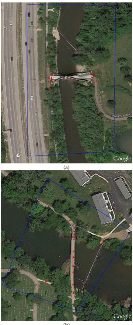
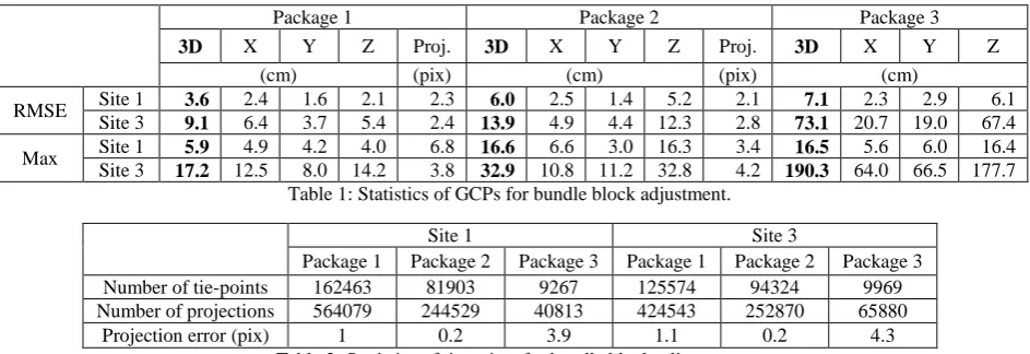
Numerous GCPs were GPS-surveyed in the area to be used in model creation. Unfortunately, the landscape of Site 2 was so hard to model that it was too difficult to find enough points with sufficient natural characteristics that could be used as GCPs. The limitations in creating the model of Site 2 meant that it was measured and modeled in a different way than the models of Sites 1 and 3, and was, therefore, left out of this analysis. Note that Sites 1 and 3 also presented problems of finding well distributed natural GCPs in the difficult to model terrain. The locations of GCPs, shown in Figure 2, were not optimal in terms of AT, though the large image overlap resulted in robust block adjustment. This allowed for assessment of the software packages in difficult circumstances. Field surveys of GCPs were executed using the GPS-RTK technique resulting in the 3D accuracy of GCPs of slightly less than 5 cm (1).
3. SOFTWARE PACKAGES AND PROCESSES
The software packages used in this analysis were treated as a black box for model creation, since in most cases the used algorithms, such as the dense matching, are proprietary and, therefore unpublished. All three packages accepted the same data inputs and generally followed the same process with differences in algorithms leading to differing degree of matching performance, and accuracy of the models. Processing in all three packages is divided into few consecutive stages that the user performed in order to generate a dense PC. The standard or default settings were used in all packages. Generally, the workflow in all three packages consisted of two separate parts: image block adjustment and dense matching. Results of both
processing parts were analyzed in this study as they provide similar parameters which helped in assessing the accuracy of the final PC models. The objective of this study was to assess the variability among different PC generating tools, as opposed to selecting which software is better than another, so the names were withheld as it may bring the wrong conclusion to the reader.
(a)
(b)
Figure 2. Location of GCPs (red triangles) and approximated image block range (blue polygon) for Sites 1 (a) and 3 (b)
4. MODEL ACCURACY ASSESSMENTS
To assess the accuracy of the models, we used two different approaches. The first approach is to analyze the statistics of the bundle adjustment, as it is the initial process, in three aspects. The first aspect is the residual of the individually measured GCPs ISPRS Annals of the Photogrammetry, Remote Sensing and Spatial Information Sciences, Volume II-1, 2014
within the model with respect to the GPS-surveyed coordinates. The second aspect is the usage and number of tie-points (TP). The third aspect is the analysis of the estimated camera calibration parameters performed during bundle adjustment. The second approach is to analyze the dense PC generation. Analysis of dense matching was performed by relatively comparing the PCs to each other including statistical and visual examination as well as through ground check point residuals.
4.1 Block Adjustment
To assess the accuracy of the block adjustment performed by the packages, an error analysis of the GCPs was performed; results are shown in Tables 1-3. First, the GCPs root-mean-squared-error (RMSE) was calculated to find the magnitude of varying quantity. This gives a good measure of the total difference or residuals between the predicted values of the location of the GCPs in the model and the observed values of the GCPs from GPS. In addition, the maximum residuals were also included to show that there were no outliers in the data. The projection error (in pixels) is included as it shows the accuracy (internal) of the block adjustment, but given in image units.
Looking at the number of TPs and projections (rays) used in AT, show the ability of each package’s algorithms to find and match the same pixels and the strength of the bundle block adjustment.
The camera self-calibration produced by each package allows for assessing of the accuracy of the built-in calibration techniques. Since the same camera is used for both test sites, each package should generally produce the same camera internal parameter results. Packages 1 and 2 provide estimates on focal length and location of the principal point (x, y), while Package 3 only provided separate focal length estimates for each image. The initial parameters were selected by each package, so they were also slightly different. Since the camera parameters estimated at both sites were quite similar for all packages they did not affect the final model created. Finally, the camera was not calibrated in a lab, therefore, it cannot be stated which calibration solution is more reliable, only circumstantial assessing can be provided.
4.2 Point Cloud
Comparing the PCs to each other can estimate the distances between points and whether there is a bias with regards to a direction or any deformation of the PCs. Secondly, point spacing shows how dense the matching is; an indicator of the performance.
Visual examination of the PCs is also beneficial as errors in the models are easily recognizable by the eye. In particular, checking the behavior of the algorithm in generating points for difficult
objects, such as dense vegetation, small parts of the bridge structure, or the extremely challenging river surface, is obvious.
The absolute accuracy of the PC geometry can be assessed using GCPs as check points since they are not used during dense matching and PC generation. Manually measuring coordinates of check points in the PC and comparing their coordinates with the GPS-surveyed reference can provide absolute errors of the PC geometry.
5. RESULTS
The models for the two sites were created based on the same images and parameters that were able to be selected in each package. There were 16 GCPs and 51 images selected for Site 1, and 15 GCPs and 47 images selected for Site 3. The ground control error/tolerance was also set the same for all software packages, at 5 cm. The identical initial conditions (as permitted by the packages) allowed for the performance comparison of the packages.
5.1 Image Block Bundle Adjustment
The statistics of the bundle block adjustment are shown in three groups. Table 1 shows the statistics for the GCPs, reporting about the model georeferencing. Table 2 shows the statistics for TPs, analyzing the matching ability of the bundle adjustment step, for each package. Table 3 shows the camera adjusted parameters.
As seen in Table 1, Site 1 had remarkably low RMSE of 3.6 cm for Package 1. This is lower than the GCPs 3D tolerance level of 5 cm, meaning that the bundle adjustment met the assumed accuracy condition. In the case of Package 2, it had a 3D accuracy slightly larger; however, it is still on the level of GCPs error tolerance. Package 3 was only slightly larger than that. The low 3D RMSE for all packages show that the GCPs while not ideally distributed provided for an accurate bundle adjustment results by all packages.
The RMSE of Packages 1 and 2 for Site 3 was 2-3 times larger than for Site 1. It was even larger for Package 3, about 10 times larger than for Site 1, with an error of 73.1 cm. Site 3 having larger errors for all packages showed that the GCP distribution for it was worse than for Site 1. Package 1 still performed well and had 3D error less than double the tolerance (10 cm), as it was the nominal goal of 2. Package 2 performed slightly worse but was still able to perform a relatively accurate bundle adjustment although larger than the nominal goal. Package 3’s model error was massive and showed that it could not perform a good bundle adjustment with the poor set of GCPs.
Package 1 Package 2 Package 3
3D X Y Z Proj. 3D X Y Z Proj. 3D X Y Z
(cm) (pix) (cm) (pix) (cm)
RMSE Site 1 3.6 2.4 1.6 2.1 2.3 6.0 2.5 1.4 5.2 2.1 7.1 2.3 2.9 6.1 Site 3 9.1 6.4 3.7 5.4 2.4 13.9 4.9 4.4 12.3 2.8 73.1 20.7 19.0 67.4
Max Site 1 5.9 4.9 4.2 4.0 6.8 16.6 6.6 3.0 16.3 3.4 16.5 5.6 6.0 16.4 Site 3 17.2 12.5 8.0 14.2 3.8 32.9 10.8 11.2 32.8 4.2 190.3 64.0 66.5 177.7
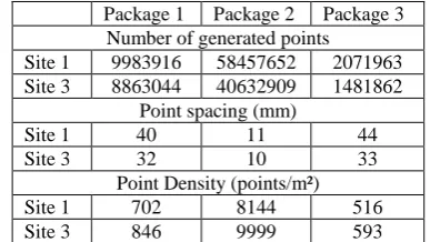
Table 1: Statistics of GCPs for bundle block adjustment.
Site 1 Site 3
Package 1 Package 2 Package 3 Package 1 Package 2 Package 3 Number of tie-points 162463 81903 9267 125574 94324 9969 Number of projections 564079 244529 40813 424543 252870 65880
Projection error (pix) 1 0.2 3.9 1.1 0.2 4.3
Table 2: Statistics of tie-points for bundle block adjustment
Package 1 Package 2 Package 3
Table 3: Statistics of camera parameters for bundle block adjustment. Note that package 3 does not adjust Principle point location. * Not estimated (equal initial values)
Judging the results, we need to consider that the test sites were selected to be quite difficult containing a river in the middle of dense canopy areas. Thus, it challenged not only the image matching algorithms but also made the collection of optimally distributed GCPs difficult to nearly impossible. Under these difficult conditions, Package 1 was able to handle the less than ideal modeling scenes and produced the most accurate block adjustment. Package 2 also performed well, just above the tolerance in Site 1 and just above the goal of 10 cm in Site 3. Package 3 fared the worst in Site 1 although still below 10 cm and had even larger errors in Site 3.
Table 1 also shows the coordinate residuals for the models. The residuals for all three axes were similar for Package 1 at both sites, meaning that the model was not biased in any direction. For Packages 2 and 3, the Z-axis residuals were larger for both sites. This error was expected to be observed since the elevation estimates of the model are more difficult to accurately calculate. This is because the accuracy of space resection and intersection included in the AT process decreases with increasing flying height. The first package having about even residuals in all components is quite impressive.
The maximum absolute residuals show that there were no gross outliers contained in the bundle adjustment which partially can prove the correctness of this process for each package.
Packages 1 and 2 Projection errors for both sites are similar and quite small considering the use of a non-metric camera.
The large number of correct TPs significantly strengthens the block geometry, but also extends the processing time. Table 2 shows that Package 1 was able to detect many more TPs than Package 2 which was still more efficient than Package 3. There is also no correlation seen between sites and number of TPs and projections. Considering the TP and projection error, it is clear that Package 3 is using the least efficient matching algorithm as not only is the number of projections the smallest, but also, it results in the largest error. Comparing accuracy of matching between the first two packages, Package 2 gives a very low projection error. This is probably explained by the threshold of matching. Package 1 may use a lower threshold resulting in a larger number of TPs but also larger projection errors whereas Package 2 may remove these matches causing lower number of projections and lower error.
Discussing results of the camera calibration process, shown in Table 3, it must be emphasized that the camera parameters were the same for each image taken over one site. The principal
distance might be different for each site, since the focusing distance was set manually, and was slightly different for each site. In the case of Package 1, the difference in estimated position of the principal point between sites is insignificant which proves that parameters were estimated properly. The principal distance was slightly larger than the initial value for Package 1 but was about the same for both sites and near the estimated value, so it is assumed to not be an error. As seen in the calibration done for both sites by Package 2, the initial parameters were very close to the final parameters; however, the x position of the principal point differed by 0.14 mm from the initial estimate, for Site 1. This offset may indicate error in the self-calibration process. In Package 3, the principal distance was estimated separately for each image, clearly causing larger errors as the difference between estimated principal distances can differ by almost 10 mm. Also, in Package 3, the principal point position is not estimated and the initial values are used; the center of the image. Unfortunately, none of the packages show the accuracy of the estimated values making it difficult to assess the reliability of the adjusted parameters.
5.2 Point Clouds Statistics
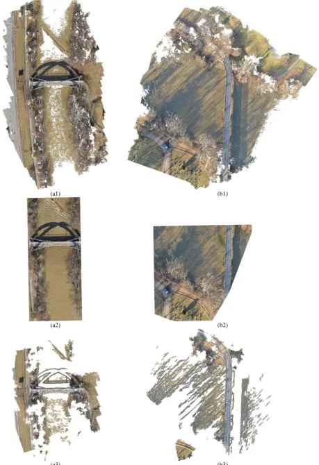
Generated PCs are dependent on the used algorithm. Top view visualization of PCs for Sites 1 and 3 are presented in Figure 3, where the relative scale within one site is preserved. Statistics of the number of total points and point spacing calculated for the models are given in the Table 4. Note that due to matching failures, e.g. on the river surface/canopy, point spacing was calculated based only on the target model areas where algorithms should work properly, e.g. on the pavement. Moreover, some of the implemented matching algorithms allow producing PCs of different densities. This parameter was chosen as default/standard since resulting density was not specified by the packages.
Package 1 Package 2 Package 3 Number of generated points
Site 1 9983916 58457652 2071963 Site 3 8863044 40632909 1481862
Point spacing (mm)
Table 4. Statistics for generated PCs for well mapped area. ISPRS Annals of the Photogrammetry, Remote Sensing and Spatial Information Sciences, Volume II-1, 2014
(a1) (b1)
(a2) (b2)
(a3) (b3)
Figure 3. Top-view of the point cloud generated for Sites 1 (a) and 3 (b) by Packages 1 (1), 2 (2), and 3 (3); note that scale is kept within the test site
For Package 1, the area covered by points is the largest. For Package 2, every ground sample has an assigned point. For Package 3, the number of points is smallest and points on the water and the ground are missing (upper and lower part of Figure 3, b3). For Package 2, the area is the smallest (strange automatic cuts to the area of interest), but the number of points, and points density is the largest; note that point spacing is even smaller than estimated GSD. Point spacing for Package 1 and 3 are similar and equal about 3-4 cm. Comparison of details mapped through different point density is shown in the Figure 4. Note that for visualization purposes, the thickness of points for each package is different due to different point spacing.
(a) (b) (c)
Figure 4. Visualization of details mapped by points for Site 3 and Packages 1 (a), 2 (b), and 3 (c) at the same scale and size
There are clearly visible difficulties in matching for Package 3, especially in shaded, dark areas where no points are matched. Package 2 uses an algorithm which finds (computes) a point for every pixel. This means that for flat, well modeled areas, such as the bridge deck in Figure 4, Package 2 will create a dense accurate PC like that of Package 1. Although in areas where matching is more difficult, Package 2 still assigns a pixel even if likely incorrect.
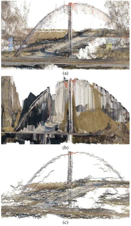
As seen best in the Figure 5, the number of wrongly matched points for Package 2 is the largest. There are not only interpolation errors, e.g. between the bridge pavement and frame (arcs), but also a lot of other points (not just on the river and canopy area) where the designated elevation is much higher or lower than the actual surface. In this case, an automatic filtering would probably fail in DSM, DTM, or object point extraction. For Package 3, the number of points is smaller and without significant errors. The visible pavement surfaces are not smooth as they should be. Package 1 shows the reasonable balance between numbers of correctly and wrongly matched points. There are small errors (e.g. on the top of the bridge frame) or points on the water (not all matched wrongly) which should be easily eliminated in the subsequent post processing. For this package, even points of small elements, such as railing on the bridge are correctly kept.
(a)
(b)
(c)
Figure 5. Isometric view of the PC of the bridge obtained using Packages 1 (a), 2 (b), and 3 (c)
Accuracy of generated PCs can be evaluated in the absolute sense, i.e. using ground check points. Due to difficulties in finding appropriate natural targets which might become check points (especially for Site 3), all GCPs used in AT were included in the set of check points. Note that the algorithm of dense point cloud generation does not require GCPs. Results of this evaluation are presented in the Table 5.
Interpreting results from Table 5, it must be emphasized that points in the PCs were selected manually based mainly on colors, as most of the check points were placed on the flat surfaces (all in the case of Site 3). The number of check points for each package was different for the same site, as not all points could be recognized and selected.
Package 1 Package 2 Package 3
3D X Y Z No. of
check points
3D X Y Z No. of
check points
3D X Y Z No. of
check points
(cm) (cm) (cm)
RMSE Site 1 12.1 5.9 7.4 7.6 28 16.2 7.9 4.2 13.5 11 26.7 7.3 6.6 24.8 26
3 8.6 4.6 4.4 5.8 15 13.4 3.3 5.6 11.7 6 51.7 8 9.2 50.2 12
Max Site 1 21.6 16.2 16.5 20 28 32.8 17.2 77 32.3 11 95.2 21.2 19.1 94.8 26
3 14.7 9.3 10.1 11.2 15 28.8 6.7 11.5 26.4 6 89.2 16.2 17 87.5 12
Table 5: Point clouds absolute accuracy.
For Site 1, some check points were placed on the corners and edges of elevation changes, which can explain the much larger errors than for Site 3 (except in Package 3 where block adjustment for Site 3 was quite inaccurate). The given values also contain interpretation errors and are affected by the PC density.
Comparing results shown in Tables 1 and 5, the same trends of accuracy are witnessed; however, the RMSE of the PCs is larger. This was expected, since the error of points selection was also added to the error of the PCs. Package 1 still exhibits no bias on the z axis while the other two packages do. Both Packages 1 and 2 have errors within acceptable ranges (2) when including the added error, for Sites 1 and 3. Package 3 still has the largest error and is outside of the acceptable error range for both sites.
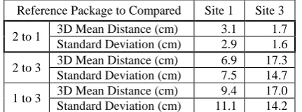
Another way of validating results might be the relative comparison of PCs, using CloudCompare (Girardeau-Montaut, 2014). This allows to see the distances between points and the variation of the measurements. The relative PCs analysis was executed only for the bridge section of each site. This resulted in comparison of the most accurate portion and target area where no large errors from the unmatchable canopy and water surface areas of the models were included. In this comparison, the most densely populated PC was set as the reference. The rationale doing this was to lower the error created from comparing against a sparse PC since distances are calculated for every point in the compared cloud. As shown in Table 6, Package 2 was used as the reference package for the comparison between it and Packages 1 and 3. Package 1 was used as the reference when comparing to Package 3.
Reference Package to Compared Site 1 Site 3
2 to 1 3D Mean Distance (cm) 3.1 1.7 Standard Deviation (cm) 2.9 1.6
2 to 3 3D Mean Distance (cm) 6.9 17.3 Standard Deviation (cm) 7.5 14.7
1 to 3 3D Mean Distance (cm) 9.4 17.0 Standard Deviation (cm) 11.1 14.2 Table 6. Cloud comparison distance and standard deviation of a well modeled area for all packages
In the distance comparison, Packages 1 and 2 were close to having their models match. This shows that these packages’ PCs were similar even with the compounding errors from bundle adjustment and PC generation in the well modeled bridge area. The comparison between Package 2 and 3 as expected from the GCP statistics was larger. While both packages modeled the area well, the offset between the whole PC compared to each other trends from the previous GCP analysis. Packages 1 and 2 were similar in the well modeled areas. Site 3 distances being smaller than Site 1 in Packages 1 and 2 was unexpected yet both errors were small enough to negate the difference from the GCP analysis and can be attributed to the smaller sample area. While Package 1 had the best bundle block adjustment, its comparison to Package 3 was worse than Package 2 comparison to Package 3. This is probably due to the elevation (Z-axis) bias found in both Packages 2 and 3. The larger elevation bias in Package 3, made its PC comparison distance further to Package 1, than 2.
6. CONCLUSION
The models created by UAS imagery can be created by a variety of UAS specific software tools. Using field data from a practically hard to model area, we were able to show the benefits and deficiencies of three different software packages. Overall, Package 1 returned the best results when looking at both bundle block adjustment results and the generated PC models for both sites. Package 2 was also effective and created accurate models just not as well as Package 1. Package 3 returned the least accurate models. These are seen in the final PC accuracy comparisons, with Packages 1 and 2 being about 10 cm and Package 3 a few tens of cm. All three packages showed that the accuracies of the models created with less than ideal data and landscapes can be close to, if not within, the error tolerances of the GPS used to collect the GCPs.
It is important to remember that this data set is difficult to model and with other data sets the results could change. The poor distribution of GCP at both sites could have contributed greatly to the amount of error seen. User deficiency in GCP selection and actual measurements are also variables that may have contributed to the error. With more data collection and field tests, comparison of the image models to each other and with models from LiDAR can all be performed to allow for a more thorough analysis of the packages. These can then help find which package and process is the most accurate and appropriate to use when modeling with low flight optical images for a specific application. UAS uses are vast and allow for the collection of survey grade spatial data whose accuracy and products must still be verified and studied in the future.
REFERENCES
Gini, R., D. Pagliari, D. Passoni, L. Pinto, G. Sona, and P. Dosso, 2013. Uav Photogrammetry: Block Triangulation Comparisons. The International Archives of the Photogrammetry, Remote Sensing and Spatial Information Sciences, Vol. XL-1/W2, pp. 157-62.
Girardeau-Montaut, D., 2014. CloudCompare - Open Source Project. http://www.danielgm.net/cc/ (accessed 09 June 2014).
Haubeck, K., and T. Prinz, 2013. A UAV-Based Low-Cost Stereo Camera System for Archaeological Surveys - Experiences from Doliche (Turkey). The International Archives of the Photogrammetry, Remote Sensing and Spatial Information Sciences, Vol. XL-1/W2, pp. 195-200.
Mikhail, E. M., Bethel J. S., and J. C. McGlone, 2001. Introduction to Modern Photogrammetry. New York: Wiley.
Niethammer, U., Rothmund, S., Schwaderer, U., Zeman, J., and M. Joswig, 2011. Open Source Image-Processing Tools For Low-Cost Uav-Based Landslide Investigations. The International Archives of the Photogrammetry, Remote Sensing and Spatial Information Sciences, Vol. XXXVIII-1/C22, pp. 161-66.
Passini, R., and K. Jacobsen, 2009. Accuracy and Radiometric Study on Very High Resolution Digital Camera Images The International Archives of the Photogrammetry, Remote Sensing and Spatial Information Sciences, Vol. XXXVIII1-4-7/W5, 6 pages (Web).
Remondino, F., Del Pizzo, S., Kersten, T., and S. Troisi, 2012. Low-cost and open-source solutions for automated image orientation – A critical overview. Proceedings EuroMed 2012 Conference, LNCS 7616, pp. 40-54.