Shafi Goldwasser
1Mihir Bellare
2July 2008
1 MIT Computer Science and Artificial Intelligence Laboratory, The Stata Center, Building 32, 32 Vassar Street, Cambridge, MA 02139, USA. E-mail:[email protected]
This is a set of lecture notes on cryptography compiled for 6.87s, a one week long course on cryptography taught at MIT by Shafi Goldwasser and Mihir Bellare in the summers of 1996–2002, 2004, 2005 and 2008.
Cryptography is of course a vast subject. The thread followed by these notes is to develop and explain the notion of provable security and its usage for the design of secure protocols.
Much of the material in Chapters 2, 3 and 7 is a result of scribe notes, originally taken by MIT graduate students who attended Professor Goldwasser’sCryptography and Cryptanalysiscourse over the years, and later edited by Frank D’Ippolito who was a teaching assistant for the course in 1991. Frank also contributed much of the advanced number theoretic material in the Appendix. Some of the material in Chapter 3 is from the chapter on Cryptography, by R. Rivest, in the Handbook of Theoretical Computer Science. Chapters 4, 5, 6, 8, 9 and 11, and Sections 10.5 and 7.4.6, are from theIntroduction to Modern Cryptography notes by Bellare and Rogaway [23], and we thank Phillip Rogaway for permission to include this material. Rosario Gennaro (as Teaching Assistant for the course in 1996) contributed Section 10.6, Section 12.4, Section 12.5, and Appendix D to the notes, and also compiled, from various sources, some of the problems in Appendix E.
All rights reserved.
Shafi Goldwasser and Mihir Bellare Cambridge, Massachusetts, July 2008.
1 Introduction to Modern Cryptography 11
1.1 Encryption: Historical Glance . . . 11
1.2 Modern Encryption: A Computational Complexity Based Theory . . . 12
1.3 A Short List of Candidate One Way Functions . . . 13
1.4 Security Definitions . . . 14
1.5 The Model of Adversary . . . 15
1.6 Road map to Encryption . . . 15
2 One-way and trapdoor functions 16 2.1 One-Way Functions: Motivation . . . 16
2.2 One-Way Functions: Definitions . . . 17
2.2.1 (Strong) One Way Functions . . . 17
2.2.2 Weak One-Way Functions . . . 18
2.2.3 Non-Uniform One-Way Functions . . . 19
2.2.4 Collections Of One Way Functions . . . 20
2.2.5 Trapdoor Functions and Collections . . . 21
2.3 In Search of Examples . . . 22
2.3.1 The Discrete Logarithm Function . . . 23
2.3.2 The RSA function . . . 26
2.3.3 Connection Between The Factorization Problem And Inverting RSA . . . 28
2.3.4 The Squaring Trapdoor Function Candidate by Rabin . . . 29
2.3.5 A Squaring Permutation as Hard to Invert as Factoring . . . 32
2.4 Hard-core Predicate of a One Way Function . . . 33
2.4.1 Hard Core Predicates for General One-Way Functions . . . 34
2.4.2 Bit Security Of The Discrete Logarithm Function . . . 35
2.4.3 Bit Security of RSA and SQUARING functions . . . 36
2.5 One-Way and Trapdoor Predicates . . . 36
2.5.1 Examples of Sets of Trapdoor Predicates . . . 37
3 Pseudo-random bit generators 39 3.0.2 Generating Truly Random bit Sequences . . . 39
3.0.3 Generating Pseudo-Random Bit or Number Sequences . . . 40
3.0.4 Provably Secure Pseudo-Random Generators: Brief overview . . . 41
3.1 Definitions . . . 41
3.2 The Existence Of A Pseudo-Random Generator . . . 42
3.3 Next Bit Tests . . . 45
3.4 Examples of Pseudo-Random Generators . . . 47
3.4.1 Blum/Blum/Shub Pseudo-Random Generator . . . 47
4 Block ciphers 48 4.1 What is a block cipher? . . . 48
4.2 Data Encryption Standard (DES) . . . 49
4.2.1 A brief history . . . 49
4.2.2 Construction . . . 49
4.2.3 Speed . . . 51
4.3 Key recovery attacks on block ciphers . . . 52
4.4 Iterated-DES and DESX . . . 55
4.4.1 Double-DES . . . 55
4.4.2 Triple-DES . . . 56
4.4.3 DESX . . . 57
4.4.4 Why a new cipher? . . . 57
4.5 Advanced Encryption Standard (AES) . . . 57
4.6 Limitations of key-recovery based security . . . 61
4.7 Problems . . . 61
5 Pseudo-random functions 63 5.1 Function families . . . 63
5.2 Random functions and permutations . . . 64
5.2.1 Random functions . . . 64
5.2.2 Random permutations . . . 66
5.3 Pseudorandom functions . . . 68
5.4 Pseudorandom permutations . . . 70
5.4.1 PRP under CPA . . . 70
5.4.2 PRP under CCA . . . 71
5.4.3 Relations between the notions . . . 72
5.5 Modeling block ciphers . . . 72
5.6 Example Attacks . . . 73
5.7 Security against key recovery . . . 75
5.8 The birthday attack . . . 78
5.9 The PRP/PRF switching lemma . . . 80
5.10 Sequences of families of PRFs and PRPs . . . 80
5.11 Some applications of PRFs . . . 81
5.11.1 Cryptographically Strong Hashing . . . 81
5.11.2 Prediction . . . 81
5.11.3 Learning . . . 82
5.11.4 Identify Friend or Foe . . . 82
5.11.5 Private-Key Encryption . . . 82
5.12 Historical notes . . . 82
6 Private-key encryption 85
6.1 Symmetric encryption schemes . . . 85
6.2 Some symmetric encryption schemes . . . 86
6.2.1 The one-time-pad encryption scheme . . . 87
6.2.2 Some modes of operation . . . 87
6.3 Issues in privacy . . . 90
6.4 Indistinguishability under chosen-plaintext attack . . . 92
6.4.1 Definition . . . 92
6.4.2 Alternative interpretation . . . 95
6.4.3 Why is this a good definition? . . . 96
6.5 Example chosen-plaintext attacks . . . 96
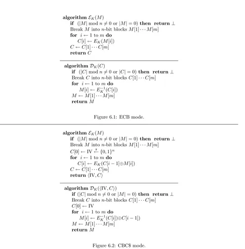
6.5.1 Attack on ECB . . . 96
6.5.2 Any deterministic, stateless schemes is insecure . . . 97
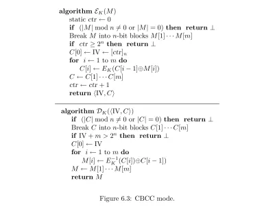
6.5.3 Attack on CBC encryption with counter IV . . . 98
6.6 IND-CPA implies PR-CPA . . . 99
6.7 Security of CTR modes . . . 101
6.7.1 Proof of Theorem?? . . . 102
6.7.2 Proof of Theorem?? . . . 106
6.8 Security of CBC with a random IV . . . 111
6.9 Indistinguishability under chosen-ciphertext attack . . . 111
6.10 Example chosen-ciphertext attacks . . . 113
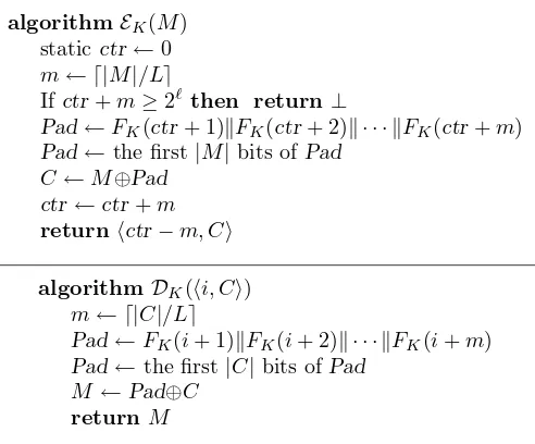
6.10.1 Attacks on the CTR schemes . . . 113
6.10.2 Attack on CBC$ . . . 114
6.11 Other methods for symmetric encryption . . . 116
6.11.1 Generic encryption with pseudorandom functions . . . 116
6.11.2 Encryption with pseudorandom bit generators . . . 117
6.11.3 Encryption with one-way functions . . . 117
6.12 Historical notes . . . 118
6.13 Problems . . . 118
7 Public-key encryption 119 7.1 Definition of Public-Key Encryption . . . 119
7.2 Simple Examples of PKC: The Trapdoor Function Model . . . 121
7.2.1 Problems with the Trapdoor Function Model . . . 121
7.2.2 Problems with Deterministic Encryption in General . . . 121
7.2.3 The RSA Cryptosystem . . . 122
7.2.4 Rabin’s Public key Cryptosystem . . . 124
7.2.5 Knapsacks . . . 125
7.3 Defining Security . . . 125
7.3.1 Definition of Security: Polynomial Indistinguishability . . . 125
7.3.2 Another Definition: Semantic Security . . . 126
7.4 Probabilistic Public Key Encryption . . . 127
7.4.1 Encrypting Single Bits: Trapdoor Predicates . . . 127
7.4.2 Encrypting Single Bits: Hard Core Predicates . . . 128
7.4.3 General Probabilistic Encryption . . . 129
7.4.4 Efficient Probabilistic Encryption . . . 130
7.4.5 An implementation of EPE with cost equal to the cost of RSA . . . 131
7.4.7 Enhancements . . . 134
7.5 Exploring Active Adversaries . . . 134
8 Hash Functions 136 8.1 The hash functionSHA1 . . . 136
8.2 Collision-resistant hash functions . . . 138
8.3 Collision-finding attacks . . . 140
8.4 One-wayness of collision-resistant hash functions . . . 142
8.5 The MD transform . . . 145
8.6 Collision-resistance under hidden-key attack . . . 147
8.7 Problems . . . 148
9 Message authentication 149 9.1 The setting . . . 149
9.2 Privacy does not imply authenticity . . . 151
9.3 Syntax of message-authentication schemes . . . 152
9.4 A definition of security for MACs . . . 153
9.4.1 Towards a definition of security . . . 153
9.4.2 Definition of security . . . 155
9.5 Examples . . . 157
9.6 The PRF-as-a-MAC paradigm . . . 159
9.7 The CBC MACs . . . 160
9.7.1 The basic CBC MAC . . . 160
9.7.2 Birthday attack on the CBC MAC . . . 161
9.7.3 Length Variability . . . 163
9.8 MACing with cryptographic hash functions . . . 164
9.8.1 The HMAC construction . . . 164
9.8.2 Security of HMAC . . . 165
9.8.3 Resistance to known attacks . . . 166
9.9 Universal hash based MACs . . . 166
9.10 Minimizing assumptions for MACs . . . 167
9.11 Problems . . . 167
10 Digital signatures 168 10.1 The Ingredients of Digital Signatures . . . 168
10.2 Digital Signatures: the Trapdoor Function Model . . . 169
10.3 Defining and Proving Security for Signature Schemes . . . 170
10.3.1 Attacks Against Digital Signatures . . . 170
10.3.2 The RSA Digital Signature Scheme . . . 171
10.3.3 El Gamal’s Scheme . . . 171
10.3.4 Rabin’s Scheme . . . 172
10.4 Probabilistic Signatures . . . 173
10.4.1 Claw-free Trap-door Permutations . . . 174
10.4.2 Example: Claw-free permutations exists if factoring is hard . . . 174
10.4.3 How to sign one bit . . . 175
10.4.4 How to sign a message . . . 176
10.4.5 A secure signature scheme based on claw free permutations . . . 177
10.5 Concrete security and Practical RSA based signatures . . . 182
10.5.1 Digital signature schemes . . . 183
10.5.2 A notion of security . . . 184
10.5.3 Generation of RSA parameters . . . 185
10.5.4 One-wayness problems . . . 187
10.5.5 Trapdoor signatures . . . 188
10.5.6 The hash-then-invert paradigm . . . 189
10.5.7 The PKCS #1 scheme . . . 191
10.5.8 The FDH scheme . . . 192
10.5.9 PSS0: A security improvement . . . 197
10.5.10 The Probabilistic Signature Scheme –PSS. . . 201
10.5.11 Signing with Message Recovery –PSS-R . . . 202
10.5.12 How to implement the hash functions . . . 203
10.5.13 Comparison with other schemes . . . 203
10.6 Threshold Signature Schemes . . . 204
10.6.1 Key Generation for a Threshold Scheme . . . 205
10.6.2 The Signature Protocol . . . 205
11 Key distribution 206 11.1 Diffie Hellman secret key exchange . . . 206
11.1.1 The protocol . . . 206
11.1.2 Security against eavesdropping: The DH problem . . . 206
11.1.3 The DH cryptosystem . . . 207
11.1.4 Bit security of the DH key . . . 207
11.1.5 The lack of authenticity . . . 208
11.2 Session key distribution . . . 208
11.2.1 Trust models and key distribution problems . . . 209
11.2.2 History of session key distribution . . . 210
11.2.3 An informal description of the problem . . . 211
11.2.4 Issues in security . . . 211
11.2.5 Entity authentication versus key distribution . . . 212
11.3 Three party session key distribution . . . 212
11.4 Authenticated key exchanges . . . 214
11.4.1 The symmetric case . . . 215
11.4.2 The asymmetric case . . . 216
11.5 Forward secrecy . . . 217
12 Protocols 219 12.1 Some two party protocols . . . 219
12.1.1 Oblivious transfer . . . 219
12.1.2 Simultaneous contract signing . . . 220
12.1.3 Bit Commitment . . . 220
12.1.4 Coin flipping in a well . . . 221
12.1.5 Oblivious circuit evaluation . . . 221
12.1.6 Simultaneous Secret Exchange Protocol . . . 222
12.2 Zero-Knowledge Protocols . . . 222
12.2.1 Interactive Proof-Systems(IP) . . . 223
12.2.3 Zero-Knowledge . . . 225
12.2.4 Definitions . . . 225
12.2.5 If there exists one way functions, then NP is in KC[0] . . . 226
12.2.6 Applications to User Identification . . . 226
12.3 Multi Party protocols . . . 227
12.3.1 Secret sharing . . . 227
12.3.2 Verifiable Secret Sharing . . . 227
12.3.3 Anonymous Transactions . . . 228
12.3.4 Multiparty Ping-Pong Protocols . . . 228
12.3.5 Multiparty Protocols When Most Parties are Honest . . . 228
12.4 Electronic Elections . . . 229
12.4.1 The Merritt Election Protocol . . . 229
12.4.2 A fault-tolerant Election Protocol . . . 230
12.4.3 The protocol . . . 231
12.4.4 Uncoercibility . . . 233
12.5 Digital Cash . . . 233
12.5.1 Required properties for Digital Cash . . . 233
12.5.2 A First-Try Protocol . . . 234
12.5.3 Blind signatures . . . 234
12.5.4 RSA blind signatures . . . 235
12.5.5 Fixing the dollar amount . . . 235
12.5.6 On-line digital cash . . . 236
12.5.7 Off-line digital cash . . . 236
A The birthday problem 249 A.1 The birthday problem . . . 249
B Some complexity theory background 251 B.1 Complexity Classes and Standard Definitions . . . 251
B.1.1 Complexity Class P . . . 251
B.1.2 Complexity Class NP . . . 251
B.1.3 Complexity Class BPP . . . 252
B.2 Probabilistic Algorithms . . . 252
B.2.1 Notation For Probabilistic Turing Machines . . . 252
B.2.2 Different Types of Probabilistic Algorithms . . . 253
B.2.3 Non-Uniform Polynomial Time . . . 253
B.3 Adversaries . . . 253
B.3.1 Assumptions To Be Made . . . 254
B.4 Some Inequalities From Probability Theory . . . 254
C Some number theory background 255 C.1 Groups: Basics . . . 255
C.2 Arithmatic of numbers: +, *, GCD . . . 256
C.3 Modular operations and groups . . . 256
C.3.1 Simple operations . . . 256
C.3.2 The main groups: Zn andZn∗ . . . 257
C.3.3 Exponentiation . . . 257
C.5 Primitive elements andZp∗ . . . 260
C.5.1 Definitions . . . 260
C.5.2 The groupZp∗ . . . 261
C.5.3 Finding generators . . . 261
C.6 Quadratic residues . . . 261
C.7 Jacobi Symbol . . . 262
C.8 RSA . . . 263
C.9 Primality Testing . . . 263
C.9.1 PRIMES∈NP . . . 263
C.9.2 Pratt’s Primality Test . . . 264
C.9.3 Probabilistic Primality Tests . . . 264
C.9.4 Solovay-Strassen Primality Test . . . 264
C.9.5 Miller-Rabin Primality Test . . . 266
C.9.6 Polynomial Time Proofs Of Primality . . . 267
C.9.7 An Algorithm Which Works For Some Primes . . . 267
C.9.8 Goldwasser-Kilian Primality Test . . . 267
C.9.9 Correctness Of The Goldwasser-Kilian Algorithm . . . 268
C.9.10 Expected Running Time Of Goldwasser-Kilian . . . 269
C.9.11 Expected Running Time On Nearly All Primes . . . 269
C.10 Factoring Algorithms . . . 270
C.11 Elliptic Curves . . . 270
C.11.1 Elliptic Curves OverZn . . . 271
C.11.2 Factoring Using Elliptic Curves . . . 272
C.11.3 Correctness of Lenstra’s Algorithm . . . 273
C.11.4 Running Time Analysis . . . 273
D About PGP 275 D.1 Authentication . . . 275
D.2 Privacy . . . 275
D.3 Key Size . . . 276
D.4 E-mail compatibility . . . 276
D.5 One-time IDEA keys generation . . . 276
D.6 Public-Key Management . . . 276
E Problems 278 E.1 Secret Key Encryption . . . 278
E.1.1 DES . . . 278
E.1.2 Error Correction in DES ciphertexts . . . 278
E.1.3 Brute force search in CBC mode . . . 278
E.1.4 E-mail . . . 279
E.2 Passwords . . . 279
E.3 Number Theory . . . 280
E.3.1 Number Theory Facts . . . 280
E.3.2 Relationship between problems . . . 280
E.3.3 Probabilistic Primality Test . . . 280
E.4 Public Key Encryption . . . 281
E.4.1 Simple RSA question . . . 281
E.4.3 Protocol Failure involving RSA . . . 281
E.4.4 RSA for paranoids . . . 281
E.4.5 Hardness of Diffie-Hellman . . . 282
E.4.6 Bit commitment . . . 282
E.4.7 Perfect Forward Secrecy . . . 282
E.4.8 Plaintext-awareness and non-malleability . . . 282
E.4.9 Probabilistic Encryption . . . 283
E.5 Secret Key Systems . . . 283
E.5.1 Simultaneous encryption and authentication . . . 283
E.6 Hash Functions . . . 284
E.6.1 Birthday Paradox . . . 284
E.6.2 Hash functions from DES . . . 284
E.6.3 Hash functions from RSA . . . 284
E.7 Pseudo-randomness . . . 284
E.7.1 Extending PRGs . . . 284
E.7.2 From PRG to PRF . . . 285
E.8 Digital Signatures . . . 285
E.8.1 Table of Forgery . . . 285
E.8.2 ElGamal . . . 285
E.8.3 Suggested signature scheme . . . 285
E.8.4 Ong-Schnorr-Shamir . . . 286
E.9 Protocols . . . 286
E.9.1 Unconditionally Secure Secret Sharing . . . 286
E.9.2 Secret Sharing with cheaters . . . 286
E.9.3 Zero–Knowledge proof for discrete logarithms . . . 286
E.9.4 Oblivious Transfer . . . 287
E.9.5 Electronic Cash . . . 287
E.9.6 Atomicity of withdrawal protocol . . . 288
Introduction to Modern Cryptography
Cryptography is about communication in the presence of an adversary. It encompasses many problems (encryp-tion, authentica(encryp-tion, key distribution to name a few). The field of modern cryptography provides a theoretical foundation based on which we may understand what exactly these problems are, how to evaluate protocols that purport to solve them, and how to build protocols in whose security we can have confidence. We introduce the basic issues by discussing the problem of encryption.
1.1
Encryption: Historical Glance
The most ancient and basic problem of cryptography is secure communication over an insecure channel. Party
Awants to send to partyB a secret message over a communication line which may be tapped by an adversary. The traditional solution to this problem is called private key encryption. In private key encryption A and B
hold a meeting before the remote transmission takes place and agree on a pair of encryption and decryption algorithms E and D, and an additional piece of information S to be kept secret. We shall refer to S as the
common secret key. The adversary may know the encryption and decryption algorithmsE and D which are being used, but does not knowS.
After the initial meeting when A wants to send B the cleartext or plaintext message m over the insecure communication line, Aencrypts mby computing the ciphertext c =E(S, m) and sends cto B. Upon receipt,
B decrypts cby computingm=D(S, c). The line-tapper (or adversary), who does not knowS, should not be able to compute mfromc.
Let us illustrate this general and informal setup with an example familiar to most of us from childhood, the
substitution cipher. In this method Aand B meet and agree on some secret permutation f: Σ→Σ (where Σ is the alphabet of the messages to be sent). To encrypt message m =m1. . . mn where mi ∈Σ, A computes
E(f, m) =f(m1). . . f(mn). To decryptc=c1. . . cn whereci∈Σ,B computesD(f, c) =f−1(c1). . . f−1(cn) =
m1. . . mn=m. In this example the common secret key is the permutationf. The encryption and decryption
algorithms E and Dare as specified, and are known to the adversary. We note that the substitution cipher is easy to break by an adversary who sees a moderate (as a function of the size of the alphabet Σ) number of ciphertexts.
A rigorous theory of perfect secrecy based on information theory was developed by Shannon [192] in 1943. 1. In
this theory, the adversary is assumed to have unlimited computational resources. Shannon showed that secure (properly defined) encryption system can exist only if the size of the secret informationS that AandB agree on prior to remote transmission is as large as the number of secret bits to be ever exchanged remotely using the encryption system.
1Shannon’s famous work on information theory was an outgrowth of his work on security ([193]).
An example of a private key encryption method which is secure even in presence of a computationally unbounded adversary is the one time pad. A andB agree on a secret bit stringpad =b1b2. . . bn, wherebi ∈R {0,1} (i.e
pad is chosen in {0,1}n with uniform probability). This is the common secret key. To encrypt a message
m = m1m2. . . mn where mi ∈ {0,1}, A computes E(pad, m) = m⊕pad (bitwise exclusive or). To decrypt
ciphertextc∈ {0,1}n,B computes
D(pad, c) =pad⊕c=pad⊕(m⊕pad) =m. It is easy to verify that∀m, c
thePrpad[E(pad, m) =c] = 21n. From this, it can be argued that seeingc gives “no information” about what
has been sent. (In the sense that the adversary’s a posteriori probability of predicting m givenc is no better than her a priori probability of predictingmwithout being givenc.)
Now, suppose Awants to sendB an additional messagem′. IfAwere to simply sendc=E(pad, m′), then the sum of the lengths of messagesm andm′ will exceed the length of the secret keypad, and thus by Shannon’s theory the system cannot be secure. Indeed, the adversary can computeE(pad, m)⊕ E(pad, m′) =m⊕m′which gives information aboutmandm′ (e.g. can tell which bits ofmandm‘ are equal and which are different). To
fix this, the length of thepadagreed upon a-priori should be the sum total of the length of all messages ever to be exchanged over the insecure communication line.
1.2
Modern Encryption: A Computational Complexity Based
The-ory
Modern cryptography abandons the assumption that the Adversary has available infinite computing resources, and assumes instead that the adversary’s computation is resource bounded in some reasonable way. In particular, in these notes we will assume that the adversary is a probabilistic algorithm who runs in polynomial time. Similarly, the encryption and decryption algorithms designed are probabilistic and run in polynomial time. The running time of the encryption, decryption, and the adversary algorithms are all measured as a function of a security parameter k which is a parameter which is fixed at the time the cryptosystem is setup. Thus, when we say that the adversary algorithm runs in polynomial time, we mean time bounded by some polynomial function ink.
Accordingly, in modern cryptography, we speak of the infeasibility of breaking the encryption system and computing information about exchanged messages where as historically one spoke of theimpossibilityof breaking the encryption system and finding information about exchanged messages. We note that the encryption systems which we will describe and claim “secure” with respect to the new adversary are not “secure” with respect to a computationally unbounded adversary in the way that the one-time pad system was secure against an unbounded adversary. But, on the other hand, it is no longer necessarily true that the size of the secret key that A and
B meet and agree on before remote transmission must be as long as the total number of secret bits ever to be exchanged securely remotely. In fact, at the time of the initial meeting, A and B do not need to know in advance how many secret bits they intend to send in the future.
We will show how to construct such encryption systems, for which the number of messages to be exchanged securely can be a polynomial in the length of the common secret key. How we construct them brings us to anther fundamental issue, namely that of cryptographic, or complexity, assumptions.
As modern cryptography is based on a gap between efficient algorithms for encryption for the legitimate users versus the computational infeasibility of decryption for the adversary, it requires that one have available prim-itives with certain special kinds of computational hardness properties. Of these, perhaps the most basic is a
one-way function. Informally, a function is one-way if it is easy to compute but hard to invert. Other primi-tives includepseudo-random number generators, andpseudorandom function families, which we will define and discuss later. From such primitives, it is possible to build secure encryption schemes.
We shall elaborate on various constructions of private-key encryption algorithms later in the course.
The development of public key cryptography in the seventies enables one to drop the requirement that A and
B must share a key in order to encrypt. The receiver B can publish authenticated2 information (called the
public-key) for anyone including the adversary, the senderA, and any other sender to read at their convenience (e.g in a phone book). We will show encryption algorithms in which whoever can read the public key can send encrypted messages to B without ever having metB in person. The encryption system is no longer intended to be used by a pair of prespecified users, but by many senders wishing to send secret messages to a single recipient. The receiver keeps secret (to himself alone!) information (called the receiver’sprivate key) about the public-key, which enables him to decrypt the cyphertexts he receives. We call such an encryption methodpublic key encryption.
We will show that secure public key encryption is possible given a trapdoor function. Informally, a trapdoor function is a one-way function for which there exists some trapdoor information known to the receiver alone, with which the receiver can invert the function. The idea of public-key cryptosystems and trapdoor functions was introduced in the seminal work of Diffie and Hellman in 1976 [71, 72]. Soon after the first implementations of their idea were proposed in [176], [170], [143].
A simple construction of public key encryption from trapdoor functions goes as follows. RecipientB can choose at random a trapdoor function f and its associated trapdoor information t, and set its public key to be a description off and its private key to bet. If Awants to send messagemtoB,AcomputesE(f, m) =f(m). To decryptc=f(m),B computesf−1(c) =f−1(f(m)) =m. We will show that this construction is not secure
enough in general, but construct probabilistic variants of it which are secure.
1.3
A Short List of Candidate One Way Functions
As we said above, the most basic primitive for cryptographic applications is a one-way function which is “easy” to compute but “hard” to invert. (For public key encryption, it must also have a trapdoor.) By “easy”, we mean that the function can be computed by a probabilistic polynomial time algorithm, and by “hard” that any probabilistic polynomial time (PPT) algorithm attempting to invert it will succeed with “small” probability (where the probability ranges over the elements in the domain of the function.) Thus, to qualify as a potential candidate for a one-way function, the hardness of inverting the function should not hold only on rare inputs to the function but with high probability over the inputs.
Several candidates which seem to posses the above properties have been proposed.
1. Factoring. The function f : (x, y) 7→ xy is conjectured to be a one way function. The asymptotically proven fastest factoring algorithms to date are variations on Dixon’s random squares algorithm [131]. It is a randomized algorithm with running timeL(n)√2whereL(n) =e√lognlog logn. The number field sieve
by Lenstra, Lenstra, Manasee, and Pollard with modifications by Adlemann and Pomerance is a factoring algorithm proved under a certain set of assumptions to factor integers in expected time
e((c+o(1))(logn) 1
3(log logn)23)
[133, 3].
2. The discrete log problem. Let pbe a prime. The multiplicative group Z∗
p = ({x < p|(x, p) = 1},·modp)
is cyclic, so thatZ∗
p ={gimodp|1≤i≤p−1}for some generatorg∈ Zp∗ . The functionf : (p, g, x)7→
(gxmodp, p, g) where pis a prime and g is a generator forZ∗
p is conjectured to be a one-way function.
Computing f(p, g, x) can be done in polynomial time using repeated squaring. However, The fastest known proved solution for its inverse, called the discrete log problem is the index-calculus algorithm, with expected running timeL(p)√2 (see [131]). An interesting problem is to find an algorithm which will
generate a primepand a generatorg forZp∗. It is not known how to find generators in polynomial time.
However, in [8], E. Bach shows how to generate random factored integers (in a given range N2 . . . N).
Coupled with a fast primality tester (as found in [131], for example), this can be used to efficiently generate random tuples (p−1, q1, . . . , qk) with p prime. Then picking g ∈ Zp∗ at random, it can be
checked if (g, p−1) = 1, ∀qi, g
p−1
qi modp 6= 1, and gp−1modp = 1, in which case order(g) = p−1
(order(g) =|{gimodp
|1≤i≤p−1}|). It can be shown that the density ofZ∗
p generators is high so that
few guesses are required. The problem of efficiently finding a generator for a specificZ∗
p is an intriguing
open research problem.
3. Subset sum. Let ai ∈ {0,1}n, ~a = (a1, . . . , an), si ∈ {0,1}, ~s = (s1, . . . , sn), and let f : (~a, ~s) 7→
(~a,Pni=1siai). An inverse of (~a,Pni=1siai) under f is any (~a, ~s′i) so that
Pn
i=1siai = Pni=1s′iai. This
function f is a candidate for a one way function. The associated decision problem (given (~a, y), does there exists~sso that Pni=1siai =y?) is NP-complete. Of course, the fact that the subset-sum problem
is NP-complete cannot serve as evidence to the one-wayness offss. On the other hand, the fact that the
subset-sum problem is easy for special cases (such as “hidden structure” and low density) can not serve as evidence for the weakness of this proposal. The conjecture thatf is one-way is based on the failure of known algorithm to handle random high density instances. Yet, one has to admit that the evidence in favor of this candidate is much weaker than the evidence in favor of the two previous ones.
4. DES with fixed message. Fix a 64 bit message M and define the functionf(K) = DESK(M) which takes
a 56 bit keyK to a 64 bit outputf(K). This appears to be a one-way function. Indeed, this construction can even be proven to be one-way assuming DES is a family of pseudorandom functions, as shown by Luby and Rackoff [139].
5. RSA. This is a candidate one-way trapdoor function. Let N = pq be a product of two primes. It is believed that such anN is hard to factor. The function isf(x) =xemodN whereeis relatively prime to
(p−1)(q−1). The trapdoor is the primesp, q, knowledge of which allows one to invert f efficiently. The functionf seems to be one-way. To date the best attack is to try to factorN, which seems computationally infeasible.
In Chapter 2 we discuss formal definitions of one-way functions and are more precise about the above construc-tions.
1.4
Security Definitions
So far we have used the terms “secure” and “break the system” quite loosely. What do we really mean? It is clear that a minimal requirement of security would be that: any adversary who can see the ciphertext and knows which encryption and decryption algorithms are being used, can not recover the entire cleartext. But, many more properties may be desirable. To name a few:
1. It should be hard to recover the messages from the ciphertext when the messages are drawn from arbitrary probability distributions defined on the set of all strings (i.e arbitrarymessage spaces). A few examples of message spaces are: the English language, the set{0,1}). We must assume that the message space is known to the adversary.
2. It should be hard to compute partial information about messages from the ciphertext.
3. It should be hard to detect simple but useful facts about traffic of messages, such as when the same message is sent twice.
4. The above properties should hold with high probability.
In short, it would be desirable for the encryption scheme to be the mathematical analogy of opaque envelopes containing a piece of paper on which the message is written. The envelopes should be such that all legal senders can fill it, but only the legal recipient can open it.
• How can “opaque envelopes” be captured in a precise mathematical definition? Much of Chapters 6 and 7 is dedicated to discussing the precise definition of security in presence of a computationally bounded adversary.
• Are “opaque envelopes” achievable mathematically? The answer is positive . We will describe the the proposals of private (and public) encryption schemes which we prove secure under various assumptions. We note that the simple example of a public-key encryptions system based on trapdoor function, described in the previous section, does not satisfy the above properties. We will show later, however, probabilistic variants of the simple system which do satisfy the new security requirements under the assumption that trapdoor functions exist. More specifically, we will show probabilistic variants of RSA which satisfy the new security requirement under, the assumption that the original RSA function is a trapdoor function, and are similar in efficiency to the original RSA public-key encryption proposal.
1.5
The Model of Adversary
The entire discussion so far has essentially assumed that the adversary can listen to cyphertexts being exchanged over the insecure channel, read the public-file (in the case of public-key cryptography), generate encryptions of any message on his own (for the case of public-key encryption), and perform probabilistic polynomial time computation. This is called apassive adversary.
One may imagine a more powerful adversary who can intercept messages being transmitted from sender to receiver and either stop their delivery all together or alter them in some way. Even worse, suppose the adversary can request a polynomial number of cyphertexts to be decrypted for him. We can still ask whether there exists encryption schemes (public or secret) which are secure against such more powerful adversaries.
Indeed, such adversaries have been considered and encryption schemes which are secure against them designed. The definition of security against such adversaries is more elaborate than for passive adversaries.
In Chapters 6 and 7 we consider a passive adversary who knows the probability distribution over the message space. We will also discuss more powerful adversaries and appropriate definitions of security.
1.6
Road map to Encryption
To summarize the introduction, our challenge is to design both secure private-key and public-key encryption systems which provably meet our definition of security and in which the operations of encryption and decryption are as fast as possible for the sender and receiver.
Chapters 6 and 7 embark on an in depth investigation of the topic of encryption, consisting of the following parts. For both private-key and public-key encryption, we will:
• Discuss formally how to define security in presence of a bounded adversary.
• Discuss current proposals of encryption systems and evaluate them respect to the security definition chosen.
• Describe how to design encryption systems which we can prove secure under explicit assumptions such as the existence of one-way functions, trapdoor functions, or pseudo random functions.
• Discuss efficiency aspects of encryption proposals, pointing out to possible ways to improve efficiency by performing some computations off-line, in batch mode, or in a incremental fashion.
One-way and trapdoor functions
One Way functions, namely functions that are “easy” to compute and “hard” to invert, are an extremely important cryptographic primitive. Probably the best known and simplest use of one-way functions, is for passwords. Namely, in a time-shared computer system, instead of storing a table of login passwords, one can store, for each passwordw, the valuef(w). Passwords can easily be checked for correctness at login, but even the system administrator can not deduce any user’s password by examining the stored table.
In Section 1.3 we had provided a short list of some candidate one-way functions. We now develop a theoretical treatment of the subject of one-way and trapdoor functions, and carefully examine the candidate one-way functions proposed in the literature. We will occasionaly refer to facts about number theory discussed in Chapter C.
We begin by explaining why one-way functions are of fundamental importance to cryptography.
2.1
One-Way Functions: Motivation
In this section, we provide motivation to the definition of one-way functions. We argue that the existence of one-way functions is a necessary condition to the existence of most known cryptographic primitives (including secure encryption and digital signatures). As the current state of knowledge in complexity theory does not allow to prove the existence of one-way function, even using more traditional assumptions asP 6=N P, we will have to assume the existence of one-way functions. We will later try to provide evidence to the plausibility of this assumption.
As stated in the introduction chapter, modern cryptography is based on a gap between efficient algorithms guaranteed for the legitimate user versus the unfeasibility of retrieving protected information for an adver-sary. To make the following discussion more clear, let us concentrate on the cryptographic task of secure data communication, namely encryption schemes.
In secure encryption schemes, the legitimate user is able to decipher the messages (using some private infor-mation available to him), yet for an adversary (not having this private inforinfor-mation) the task of decrypting the ciphertext (i.e., “breaking” the encryption) should be infeasible. Clearly, the breaking task can be performed by a non-deterministic polynomial-time machine. Yet, the security requirement states that breaking should not be feasible, namely could not be performed by a probabilistic polynomial-time machine. Hence, the existence of se-cure encryption schemes implies that there are tasks performed by non-deterministic polynomial-time machines yet cannot be performed by deterministic (or even randomized) polynomial-time machines. In other words, a necessary condition for the existence of secure encryption schemes is that N P is not contained in BPP (and hence thatP 6=N P).
However, the above mentioned necessary condition (e.g.,P 6=N P) is not a sufficient one. P 6=N Ponly implies
that the encryption scheme is hard to break in the worst case. It does not rule-out the possibility that the encryption scheme is easy to break in almost all cases. In fact, one can easily construct “encryption schemes” for which the breaking problem is NP-complete and yet there exist an efficient breaking algorithm that succeeds on 99% of the cases. Hence, worst-case hardness is a poor measure of security. Security requires hardness on most cases or at least average-case hardness. Hence, a necessary condition for the existence of secure encryption schemes is the existence of languages in N P which are hard on the average. Furthermore, P 6= N P is not known to imply the existence of languages inN P which are hard on the average.
The mere existence of problems (in NP) which are hard on the average does not suffice. In order to be able to use such problems we must be able to generate such hard instances together with auxiliary information which enable to solve these instances fast. Otherwise, the hard instances will be hard also for the legitimate users and they gain no computational advantage over the adversary. Hence, the existence of secure encryption schemes implies the existence of an efficient way (i.e. probabilistic polynomial-time algorithm) of generating instances with corresponding auxiliary input so that
(1) it is easy to solve these instances given the auxiliary input; and
(2) it is hard on the average to solve these instances (when not given the auxiliary input).
We avoid formulating the above “definition”. We only remark that the coin tosses used in order to generate the instance provide sufficient information to allow to efficiently solve the instance (as in item (1) above). Hence, without loss of generality one can replace condition (2) by requiring that these coin tosses are hard to retrieve from the instance. The last simplification of the above conditions essentially leads to the definition of a one-way function.
2.2
One-Way Functions: Definitions
In this section, we present several definitions of one-way functions. The first version, hereafter referred to as strong one-way function (or just one-way function), is the most convenient one. We also present weak one-way functions which may be easier to find and yet can be used to construct strong one way functios, and non-uniform one-way functions.
2.2.1
(Strong) One Way Functions
The most basic primitive for cryptographic applications is a one-way function. Informally, this is a function which is “easy” to compute but “hard” to invert. Namely, any probabilistic polynomial time (PPT) algorithm attempting to invert the one-way function on a element in its range, will succeed with no more than “negligible” probability, where the probability is taken over the elements in the domain of the function and the coin tosses of the PPT attempting the inversion.
This informal definition introduces a couple of measures that are prevalent in complexity theoretic cryptography. An easy computation is one which can be carried out by a PPT algorithm; and a functionν:N→Ris negligible if it vanishes faster than the inverse of any polynomial. More formally,
Definition 2.1 ν is negligible if for every constantc≥0 there exists an integerkc such thatν(k)< k−c for all
k≥kc.
Another way to think of it isν(k) =k−ω(1).
time”. A “strong negation” of the notion of a negligible fraction/probability is the notion of a non-negligible fraction/probability. we say that a function ν isnon-negligibleif there exists a polynomial psuch that for all sufficiently largek’s it holds thatν(k)> p(1k). Note that functions may be neither negligible nor non-negligible.
Definition 2.2 A functionf:{0,1}∗→ {0,1}∗ isone-way if:
(1) there exists a PPT that on inputxoutputf(x);
(2) For every PPT algorithmAthere is a negligible functionνA such that for sufficiently largek, Prhf(z) =y : x $
← {0,1}k ; y
←f(x) ; z←A(1k, y)i
≤ νA(k)
Remark 2.3 The guarantee is probabilistic. The adversary is not unable to invert the function, but has a low probability of doing so where the probability distribution is taken over the input x to the one-way function where xif of lengthk, and the possible coin tosses of the adversary. Namely, x is chosen at random andy is set tof(x).
Remark 2.4 The advsersary is not asked to findx; that would be pretty near impossible. It is asked to find some inverse ofy. Naturally, if the function is 1-1 then the only inverse isx.
Remark 2.5 Note that the adversary algorithm takes as inputf(x) and the security parameter 1k (expressed
in unary notatin) which corresponds to the binary length ofx. This represents the fact the adversary can work in time polynomial in |x|, even if f(x) happends to be much shorter. This rules out the possibility that a function is considered one-way merely because the inverting algorithm does not have enough time to print the output. Consider for example the function defined as f(x) =y where y is the logk least significant bits of x
where|x|=k. Since the|f(x)|= log|x|no algorithm can invertf in time polynomial in|f(x)|, yet there exists an obvious algorithm which finds an inverse off(x) in time polynomial in|x|. Note that in the special case of length preserving functionsf (i.e.,|f(x)|=|x|for allx’s), the auxiliary input is redundant.
Remark 2.6 By this definition it trivially follows that the size of the output off is bounded by a polynomial in k, sincef(x) is a poly-time computable.
Remark 2.7 The definition which is typical to definitions from computational complexity theory, works with asymptotic complexity—what happens as the size of the problem becomes large. Security is only asked to hold for large enough input lengths, namely as k goes to infinity. Per this definition, it may be entirely feasible to invert f on, say, 512 bit inputs. Thus such definitions are less directly relevant to practice, but useful for studying things on a basic level. To apply this definition to practice in cryptography we must typically envisage not a single one-way function but a family of them, parameterized by asecurity parameter k. That is, for each value of the security parameterkthere is be a specific functionf :{0,1}k→ {0,1}∗. Or, there may be a family
of functions (or cryptosystems) for each value ofk. We shall define such familes in subsequent section.
The next two sections discuss variants of the strong one-way function definition. The first time reader is encouraged to directly go to Section 2.2.4.
2.2.2
Weak One-Way Functions
One way functions come in two flavors: strong and weak. The definition we gave above, refers to a strong way function. We could weaken it by replacing the second requirement in the definition of the function by a weaker requirement as follows.
(1) there exists a PPT that on inputxoutputf(x);
(2) There is a polynomial functionsQsuch that for every PPT algorithmA, and for sufficiently large k,
Prhf(z)6=y : x← {$ 0,1}k ; y←f(x) ; z←A(1k, y)i≥ 1
Q(k)
The difference between the two definitions is that whereas we only require some non-negligible fraction of the inputs on which it is hard to invert a weak one-way function, a strong one-way function must be hard to invert on all but a negligible fraction of the inputs. Clearly, the latter is preferable, but what if only weak one-way functions exist ? Our first theorem is that the existence of a weak one way function implies the existence of a strong one way function. Moreover, we show how to construct a strong one-way function from a weak one. This is important in practice as illustarted by the following example.
Example 2.9 Consider for example the functionf :Z×Z7→Z wheref(x, y) =x·y. This function can be easily inverted on at least half of its outputs (namely, on the even integers) and thus is not a strong one way function. Still, we said in the first lecture thatf is hard to invert whenxandyare primes of roughly the same length which is the case for a polynomial fraction of thek-bit composite integers. This motivated the definition of a weak one way function. Since the probability that ank-bit integer xis prime is approximately 1/k, we get the probability that both xand y such that |x| = |y|= k are prime is approximately 1/k2. Thus, for allk,
about 1− 1
k2 of the inputs tof of length 2k are prime pairs of equal length. It is believed that no adversary
can invertf whenxandyare primes of the same length with non-negligible success probability, and under this belief,f is a weak one way function (as condition 2 in the above definition is satisfied forQ(k) =O(k2)).
Theorem 2.10 Weak one way functions exist if and only if strong one way functions exist.
Proof Sketch: By definition, a strong one way function is a weak one way function. Now assume that f is a weak one way function such thatQis the polynomial in condition 2 in the definition of a weak one way function. Define the function
f1(x1. . . xN) =f(x1). . . f(xN)
whereN = 2kQ(k) and eachxi is of lengthk.
We claim that f1 is a strong one way function. Since f1 is a concatenation of N copies of the function f, to
correctly invertf1, we need to invertf(xi) correctly for eachi. We know that every adversary has a probability
of at least Q1(k) to fail to invertf(x) (where the probability is taken overx∈ {0,1}k and the coin tosses of the
adversary), and so intuitively, to invertf1we need to invert O(kQ(k)) instances off. The probability that the
adversary will fail for at least one of these instances is extremely high.
The formal proof (which is omitted here and will be given in appendix) will take the form of a reduction; that is, we will assume for contradiction thatf1 is not a strong one way function and that there exists some adversary
A1 that violates condition 2 in the definition of a strong one way function. We will then show that A1 can be
used as a subroutine by a new adversaryA that will be able to invert the original functionf with probability better than 1− 1
Q(|x|) (where the probability is taken over the inputsx∈ {0,1}k and the coin tosses ofA). But
this will mean thatf is not a weak one way function and we have derived a contradiction.
This proof technique is quite typical of proofs presented in this course. Whenever such a proof is presented it is important to examine the cost of the reduction. For example, the construction we have just outlined is not length preserving, but expands the size of the input to the function quadratically.
2.2.3
Non-Uniform One-Way Functions
of polynomial size algorithm We stress that the “easy to compute” condition is still stated in terms of uniform algorithms. For example, following is a non-uniform version of the definition of (strong) one-way functions.
Definition 2.11 A functionf is callednon-uniformly strong one-way if the following two conditions hold
(1) easy to compute: as before There exists a PPT algorithm to compute forf.
(2) hard to invert: For every (even non-uniform) family of polynomial-size algorithms A ={Mk}k∈N, there
exists a negligbleνA such that for all sufficiently largek’s Prhf(z)6=y : x← {$ 0,1}k ; y
←f(x) ; z←Mk(y)
i
≤ νA(k)
Note that it is redundent to give 1k as an auxiliary input toM k.
It can be shown that iff is non-uniformly one-way then it is (strongly) one-way (i.e., in the uniform sense). The proof follows by converting any (uniform) probabilistic polynomial-time inverting algorithm into a non-uniform family of polynomial-size algorithm, without decreasing the success probability. Details follow. Let A′ be a
probabilistic polynomial-time (inverting) algorithm. Letrk denote a sequence of coin tosses forA′ maximizing
the success probability ofA′. The desired algorithmMk incorporates the code of algorithmA′ and the sequence
rk (which is of length polynomial ink).
It is possible, yet not very plausible, that strongly one-way functions exist and but there are no non-uniformly one-way functions.
2.2.4
Collections Of One Way Functions
Instead of talking about a single functionf :{0,1}∗→ {0,1}∗, it is often convenient to talk about collections of
functions, each defined over some finite domain and finite ranges. We remark, however, that the single function format makes it easier to prove properties about one way functions.
Definition 2.12 LetI be a set of indices and fori∈I letDiandRi be finite. A collection of strong one way
functions is a setF ={fi:Di→Ri}i∈I satisfying the following conditions. (1) There exists a PPTS1 which on input 1k outputs ani∈ {0,1}k∩I
(2) There exists a PPTS2 which on inputi∈Ioutputsx∈Di
(3) There exists a PPTA1 such that fori∈I andx∈Di,A1(i, x) =fi(x). (4) For every PPTA there exists a negligibleνA such that∀ klarge enough
Prhfi(z) =y : i
$
←I ; x $
←Di ; y←fi(x) ; z←A(i, y)
i
≤ νA(k)
(here the probability is taken over choices of iandx, and the coin tosses ofA).
In general, we can show that the existence of a single one way function is equivalent to the existence of a collection of one way functions. We prove this next.
Theorem 2.13 A collection of one way functions exists if and only if one way functions exist.
Proof:Suppose thatf is a one way function.
Set F = {fi : Di → Ri}i∈I where I = {0,1}∗ and for i ∈ I, take Di = Ri = {0,1}|i| and fi(x) = f(x).
and A1(i, x) =fi(x) =f(x). (Note thatf is polynomial time computable.) Condition 4 in the definition of a
collection of one way functions clearly follows from the similar condition forf to be a one way function. Now suppose that F = {fi : Di → Ri}i∈I is a collection of one way functions. Define fF(1k, r1, r2) =
A1(S1(1k, r1), S2(S1(1k, r1), r2)) whereA1,S1, andS2 are the functions associated withF as defined in
Defini-tion 2.12. In other words,fF takes as input a string 1k◦r1◦r2 where r1 and r2 will be the coin tosses ofS1
andS2, respectively, and then
• RunsS1on input 1k using the coin tossesr1to get the indexi=S1(1k, r1) of a functionfi∈F.
• RunsS2on the outputiofS1 using the coin tossesr2to find an inputx=S2(i, r2). • RunsA1oniandxto computefF(1k, r1, r2) =A1(i, x) =fi(x).
Note that randomization has been restricted to the input offF and sinceA1is computable in polynomial time,
the conditions of a one way function are clearly met.
A possible example is the following, treated thoroughly in Section 2.3.
Example 2.14 The hardness of computing discrete logarithms yields the following collection of functions. Define EXP ={EXPp,g(i) =gi modp, EXP p, g:Zp →Zp∗}<p,g>∈I forI ={< p, g > pprime,g generator
forZ∗
p}.
2.2.5
Trapdoor Functions and Collections
Infromally, atrapdoor functionf is a one-way function with an extra property. There also exists a secret inverse function (thetrapdoor) that allows its possessor to efficiently invertf at any point in the domain of his choosing. It should be easy to computef on any point, but infeasible to invertf on any point without knowledge of the inverse function . Moreover, it should be easy to generate matched pairs of f’s and corresponding trapdoor. Once a matched pair is generated, the publication of f should not reveal anything about how to compute its inverse on any point.
Definition 2.15 A trapdoor function is a one-way function f : {0,1}∗ → {0,1}∗ such that there exists a
polynomialpand a probabilistic polynomial time algorithmIsuch that for everykthere exists antk∈ {0,1}∗
such that|tk| ≤p(k) and for allx∈ {0,1}∗,I(f(x), tk) =y such thatf(y) =f(x).
An example of a function which may be trapdoor if factoring integers is hard was proposed by Rabin[170]. Let
f(x, n) =x2modn where n=pq a product of two primes and x ∈Z∗
n. Rabin[170] has shown that inverting
f is easy iff factoring composite numbers product of two primes is easy. The most famous candidate trapdoor function is the RSA[176] functionf(x, n, l) =xlmodnwhere (l, φ(n)) = 1.
Again it will be more convenient to speak of families of trapdoor functions parameterized by security parameter
k.
Definition 2.16 LetIbe a set of indices and fori∈IletDibe finite. A collection of strong one way trapdoor
functions is a setF ={fi:Di→Di}i∈I satisfying the following conditions.
(1) There exists a polynomial pand a PTM S1 which on input 1k outputs pairs (i, ti) wherei ∈I∩ {0,1}k
and|ti|< p(k) The informationti is referred to as the trapdoor ofi. (2) There exists a PTMS2which on input i∈I outputsx∈Di
(3) There exists a PTMA1 such that fori∈I,x∈Di A1(i, x) =fi(x).
(4) There exists a PTMA2 such thatA2(i, ti, fi(x)) =xfor allx∈Di and for alli∈I(that is,fi is easy to
(5) For every PPTA there exists a negligbleνA such that∀k large enough
Prhfi(z) =y : i
$
←I ; x←$ Di ; y←fi(x) ; z←A(i, y)
i
≤ νA(k)
A possible example is the following treated in in detail in the next sections.
Example 2.17 [The RSA collections of possible trapdoor functions ] Letp, qdenote primes,n=pq,Zn∗={1≤
x≤n,(x, n) = 1} the multiplicative group whose cardinality isϕ(n) = (p−1)(q−1), ande∈Zp−1 relatively
prime toϕ(n). Our set of indices will beI={< n, e >such thatn=pq|p|=|q|}and the trapdoor associated with the particular index< n, e >bedsuch thated= 1 modφ(n). LetRSA={RSA<n,e>:Zn∗ →Zn∗}<n,e>∈I
whereRSA<n,e>(x) =xemodn
2.3
In Search of Examples
Number theory provides a source of candidates for one way and trapdoor functions. Let us start our search for examples by a digression into number theorey. See also the mini-course on number theory in Appendix C.
Calculating Inverses in
Z
p∗Consider the set Z∗
p ={x: 1≤x < pand gcd(x, p) = 1} where pis prime. Z∗p is a group under multiplicaton
modulop. Note that to find the inverse of x∈Z∗
p; that is, an elementy ∈Z∗p such thatyx≡1 modp, we can
use the Euclidean algorithm to find integers y andz such thatyx+zp= 1 = gcd(x, p). Then, it follows that
yx≡1 modpand so ymodpis the desired inverse.
The Euler Totient Function
ϕ
(
n
)
Euler’s Totient Functionϕ is defined by ϕ(n) = |{x: 1 ≤x < pand gcd(x, n) = 1}. The following are facts aboutϕ.
(1) Forpa prime andα≥1,ϕ(pα) =pα−1(p −1).
(2) For integersm, nwith gcd(m, n) = 1,ϕ(mn) =ϕ(m)ϕ(n). Using the rules above, we can find ϕfor anynbecause, in general,
ϕ(n) = ϕ(
k
Y
i=1
piαi)
=
k
Y
i=1
ϕ(piαi)
=
k
Y
i=1
piαi−1(pi−1)
Z
p∗Is Cyclic
A groupGis cyclic if and only if there is an elementg∈Gsuch that for everya∈G, there is an integerisuch that gi=a. We callg ageneratorof the groupGand we denote the indexibyind
Theorem 2.18 (Gauss) If p is prime thenZ∗p is a cyclic group of order p−1. That is, there is an element
g∈Z∗
p such thatgp−1≡1 modpandgi6≡1 modpfori < p−1.
¿From Theorem 2.18 the following fact is immediate.
Fact 2.19 Given a primep, a generatorg forZ∗
p, and an elementa∈Z∗p, there is a unique 1≤i≤p−1 such
that a=gi.
The Legendre Symbol
Fact 2.20 Ifpis a prime andg is a generator ofZ∗p, then
gc=gagbmodp
⇔c=a+bmodp−1
¿From this fact it follows that there is an homomorphism f : Z∗
p →Zp−1 such that f(ab) =f(a) +f(b). As
a result we can work withZp−1 rather than Z∗p which sometimes simplifies matters. For example, suppose we
wish to determine how many elements inZ∗p are perfect squares (these elements will be referred to asquadratic residuesmodulop). The following lemma tells us that the number of quadratic residues modulopis 12|Z∗p|.
Lemma 2.21 a∈Z∗
pis a quadratic residue modulopif and only ifa=gxmodpwherexsatisfies 1≤x≤p−1
and is even.
Proof:Letg be a generator inZ∗p.
(⇐) Suppose an elementa=g2xfor some x. Thena=s2where s=gx.
(⇒) Consider the square of an elementb=gy. b2=g2y≡gemodpwhereeis even since 2yis reduced modulo
p−1 which is even. Therefore, only those elements which can be expressed as ge, for e an even integer, are
squares.
Consequently, the number of quadratic residues modulopis the number of elements in Z∗
p which are an even
power of some given generatorg. This number is clearly 12|Z∗p|.
TheLegendre SymbolJp(x) specifies whetherxis a perfect square inZ∗pwhere pis a prime.
Jp(x) =
1 ifxis a square inZ∗
p
0 if gcd(x, p)6= 1
−1 ifxis not a square inZ∗
p
The Legendre Symbol can be calculated in polynomial time due to the following theorem.
Theorem 2.22 [Euler’s Criterion]Jp(x)≡x
p−1
2 modp.
Using repeated doubling to compute exponentials, one can calculatexp−21 inO(|p|3) steps. Though thisJp(x)
can be calculated whenpis a prime, it is not known how to determine for generalxandn, whetherxis a square in Z∗n.
2.3.1
The Discrete Logarithm Function
Let EXP be the function defined by EXP(p, g, x) = (p, g, gxmodp). We are particularly interested in the case whenpis a prime andgis a generator ofZ∗
p. Deine an index setI={(p, g) :pis prime andg is a generator ofZp∗}.
y ∈Z∗p the discrete logarithm function DL by DL(p, g, y) = (p, g, x) wherex∈Zp−1 andgx≡ymodp. Given
pand g, EXP(p, g, x) can easily be computed in polynomial time. However, it is unknown whether or not its inverse DL can be computed in polynomial time unless p−1 has very small factors (see [164]). Pohlig and Hellman [164] present effective techniques for this problem whenp−1 has only small prime factors.
The best fully proved up-to-date algorithm for computing discrete logs is the Index-calculus algorithm. The expected running time of such algorithm is polynomial ine√klogkwherekis the size of the modulosp. There is
a recent variant of the number field sieve algorithm for discrete logarithm which seems to work in faster running time ofe(klogk)13
. It interesting to note that working over the finite fieldGF(2k) rather than working modulop
seems to make the problem substantially easier (see Coppersmith [61] and Odlyzko [158]). Curiously, computing discrete logarithms and factoring integers seem to have essentially the same difficulty at least as indicated by the current state of the art algorithms.
With all this in mind, we consider EXP a good candidate for a one way function. We make the following explicit assumption in this direction. The assumption basically says that there exists no polynomial time algorithm that can solvethe discrete log problem with prime modulos.
Strong Discrete Logarithm Assumption (DLA):1 For every polynomial Q and every PPT A, for all
sufficiently large k,
Pr[A(p, g, y) =xsuch thaty≡gxmodpwhere 1≤x≤p−1]< 1 Q(k) (where the probability is taken over all primespsuch that|p| ≤k, the generatorsg ofZ∗
p,x∈Z∗p and the coin
tosses of A).
An immediate consequence of this assumption we get
Theorem 2.23 Under the strong discrete logarithm assumption there exists a strong one way function; namely, exponentiation modulo a primep.
Some useful properties of EXP and DL follow.
Remark 2.24 If DL(p, g1, y) is easy to calculate for some generator g1 ∈Z∗p then it is also easy to calculate
DL(p, g2, y) for any other generator g2 ∈ Zp∗. (The group Z∗p has ϕ(p−1) generators.) To see this suppose
that x1= DL(p, g1, y) and x2= DL(p, g2, y). Ifg2≡g1zmodpwhere gcd(z, p−1) theny ≡g1x2zmodpand
consequently, x2≡z−1x1modp−1.
The following result shows that to efficiently calculate DL(p, g, y) for (p, g)∈Iit will suffice to find a polynomial time algorithm which can calculate DL(p, g, y) on at least a 1
Q(|p|) fraction of the possible inputs y ∈Z∗p for
some polynomialQ.
Proposition 2.25 Letǫ,δ∈(0,1) and letSbe a subset of the prime integers. Suppose there is a probabilistic algorithm A such that for all primesp∈S and for all generatorsg ofZ∗p
Pr[A(p, g, y) =xsuch thatgx≡ymodp]> ǫ
(where the probability is taken overy∈Z∗pand the coin tosses of A) and A runs in time polynomial in|p|. Then
there is a probabilistic algorithm A′ running in time polynomial in ǫ−1, δ−1, and |p| such that for all primes
1We note that a weaker assumption can be made concerning the discrete logarithm problem, and by the standard construction one can still construct a strong one-way function. We will assume for the purpose of the course the first stronger assumption.
Weak Discrete Logarithm Assumption: There is a polynomialQsuch that for every PTM A there exists an integerk0such that∀k > k0 Pr[A(p, g, y) =xsuch thaty≡gxmodpwhere 1≤x≤p−1]<1−Q(k)1 (where the probability is taken over all primespsuch that|p| ≤k, the generatorsgofZ∗p,x∈Z∗
p∈S, generatorsgofZ∗p, andy∈Z∗p
Pr[A′(p, g, y) =xsuch thatgx
≡ymodp]>1−δ
(where the probability is taken over the coin tosses of A′).
Proof:Choose the smallest integerN for which 1
eN < δ.
Consider the algorithm A′ running as follows on inputsp∈S,g a generator ofZ∗
p andy∈Z∗p.
Repeatǫ−1N times.
Randomly choose zsuch that 1≤z≤p−1. Letw=A(p, g, gzy)
IfA succeeds thengw=gzy=gz+xmodpwherex= DL p,g(y)
and therefore DLp,g(y) =w−zmodp−1.
Otherwise, continue to next iteration. End loop
We can estimate the probability that A′ fails:
Pr[A′(p, g, y) fails] = Pr[A single iteration of the loop of A′ fails]ǫ−1N
<(1−ǫ)ǫ−1N
<(e−N)
< δ
Note that since N =O(log(δ−1)) =O(δ−1), A′ is a probabilistic algorithm which runs in time polynomial in ǫ−1,δ−1, and
|p|.
The discrete logarithm problem also yields the following collection of functions. LetI={(p, g) :pis prime andg is a generator ofZ∗
p}and define
EXP ={EXPp,g:Zp−1→Z∗p where EXPp,g(x) =gxmodp}(p,g)∈I.
Then, under the strong discrete logarithm assumption, EXP is a collection of strong one way functions. This claim will be shown to be true next.
Theorem 2.26 Under the strong discrete logarithm assumption there exists a collection of strong one way functions.
Proof: We shall show that under the DLA EXP is indeed a collection of one way functions. For this we must show that it satisfies each of the conditions in the definition of a collection of one way functions.
For condition 1, defineS1to run as follows on input 1k.
(1) Run Bach’s algorithm (given in [8]) to get a random integernsuch that|n|=kalong with its factorization.
(2) Test whethern+ 1 is prime. See primality testing in section C.9.
(3) If so, letp=n+ 1. Given the prime factorization ofp−1 we look for generatorsg ofZ∗
p as follows. (1) Chooseg∈Z∗
(2) Ifp−1 =Y
i
qiαi is the prime factorization ofp−1 then for eachqi check thatg
p−1
qi 6≡1 modp.
If so, theng is a generator ofZ∗p. Outputpandg.
Otherwise, repeat from step 1.
Claim 2.27 gis a generator ofZ∗p if for each prime divisorqofp−1,g
p−1
q 6≡1 modp.
Proof:The elementgis a generator ofZ∗pifgp−1≡1 modpandgj6≡1 modpfor alljsuch that 1≤j < p−1;
that is,ghas orderp−1 inZ∗
p.
Now, suppose that g satisfies the condition of Claim 2.27 and letm be the order ofg in Z∗p. Thenm |p−1.
Ifm < p−1 then there exists a primeq such thatm| p−q1; that is, there is an integerdsuch thatmd= p−q1. Thereforegp−q1 = (gm)d≡1 modncontradicting the hypothesis. Hence,m=p−1 and gis a generator ofZ∗
p.
Also, note that the number of generators inZ∗p isϕ(p−1) and in [178] it is shown that
ϕ(k)> k
6 log logk.
Thus we expect to have to chooseO(log logp) candidates forgbefore we obtain a generator. Hence,S1runs in
expected polynomial time.
For condition 2 in the definition of a collection of one way functions, we can defineS2to simply outputx∈Zp−1
at random giveni= (p, g).
Condition 3 is true since the computation of gxmodpcan be performed in polynomial time and condition 4
follows from the strong discrete logarithm assumption.
2.3.2
The RSA function
In 1977 Rivest, Shamir, and Adleman [176] proposed trapdoor function candidate motivated by finding a public-key cryptosystem satisfying the requirements proposed by Diffie and Hellman. The trapdoor function proposed isRSA(n, e, x) =xemodnwhere the case of interest is thatnis the product of two large primespandq and
gcd(e, φ(n)) = 1. The corresponding trapdoor information isdsuch that d·e≡1 modφ(n).
Viewd as a collection, let RSA ={RSAn,e:Z∗n →Z∗n where RSAn,e(x) =xemodn}(n,e)∈I.forI ={< n, e >
s.t. n=pq|p|=|q|,(e, φ(n)) = 1} .
RSA is easy to compute. How hard is it to invert? We know that if we can factor n we can invert RSA via the Chinese Remainder Theorem, however we don’t know if the converse is true. Thus far, the best way known to invert RSA is to first factor n. There are a variety of algorithms for this task. The best running time for a fully proved algorithm is Dixon’s random squares algorithms which runs in time O(e√lognlog logn).
In practice we may consider others. Let ℓ=|p| where pis the smallest prime divisor of n. TheElliptic Curve
algorithm takes expected time O(e√2ℓlogℓ). The Quadratic Sieve algorithm runs in expected O(e√lnnln lnn).