210 (2010) 1726–1737
Contents lists available atScienceDirect
Journal of Materials Processing Technology
j o u r n a l h o m e p a g e :w w w . e l s e v i e r . c o m / l o c a t e / j m a t p r o t e c
Internal state variable plasticity-damage modeling of the copper
tee-shaped tube hydroforming process
J. Crapps
a,∗, E.B. Marin
b, M.F. Horstemeyer
a,b, R. Yassar
c, P.T. Wang
baDepartment of Mechanical Engineering, Mississippi State University, Mississippi State, MS, United States bCenter for Advanced Vehicular Systems, Mississippi State University, Mississippi State, MS, United States
cDepartment of Mechanical Engineering and Engineering Mechanics Michigan Technological University, Houghton, MI, United States
a r t i c l e
i n f o
Article history:
Received 3 June 2009
Received in revised form 25 May 2010 Accepted 2 June 2010
This paper presents a parametric finite element analysis using a history-dependent internal state vari-able model for a hydroforming process. Experiments were performed for the internal state varivari-able model correlation and for validating a 2-in. copper tee hydroforming process simulation. The material model constants were determined from uniaxial stress–strain responses obtained from tensile tests on the tube’s material. In the finite element simulations, the mesh and boundary conditions were integrated with the geometry and process parameters currently used in industry. The study provides insights for the varia-tion of different process parameters (velocity and pressure profiles, and bucking system characteristics) related to the finished product.
© 2010 Elsevier B.V. All rights reserved.
1. Introduction
Tube hydroforming is a metal forming process in which tubes are formed into complex shapes within a die cavity using inter-nal pressure and axial compressive forces simultaneously. The development of the initial techniques and establishment of the theoretical background goes back to the 1940s (Koc and Altan, 2001).Grey et al. (1939)were the first to report on hydroforming of seamless copper fittings with T-branches. According toAhmetoglu et al. (2000), tube hydroforming offers many advantages over conventional manufacturing methods including: part consolida-tion, weight reducconsolida-tion, improved structural strength and stiffness, lower tooling cost due to fewer parts, fewer secondary opera-tions, reduced dimensional variaopera-tions, and reduced scrap. They also report that most applications of tube hydroforming can be found in the auto and aircraft industries as well as manufacturing com-ponents for sanitary use.
The hydroforming process has some inherent problems that include bursting (fracture), wrinkling, and wall thinning, which strongly depend on the choice of the processing conditions. One
Abbreviations:DHP Copper, Deoxidized High Phosphorus Copper; EMMI, Evolv-ing Microstructural Model of Inelasticity; OFHC, Oxygen Free High Conductivity.
∗Corresponding author. Tel.: +1 6623123251; fax: +1 6623257223. E-mail address:[email protected](J. Crapps).
particular hydroforming process in which these inherent problems often arise is a T-branch type use for fittings. As such the focus of our study is to analyze a 2-in. copper tee forming process with a history-dependent internal state variable plasticity model to better control the process outcome.
Modeling of hydroforming via FEM has been a focal point of much recent research.Chen et al. (2000)worked to obtain a funda-mental understanding of the hydroforming process variables such as internal pressure, ram movement, and lubricant through corner fill modeling.Strano et al. (2001)used FEM to develop an adaptive simulation to select a feasible hydroforming loading path with a minimum number of runs. The adaptive technique detects the onset of defects (wrinkling, bursting, buckling) and adjusts the loading paths accordingly.Shirayori et al. (2002)investigated via FEM and experiments the free hydraulic bulging of copper and aluminum alloy tubes. They found that an increase in thickness deviation during free bulging depended on tube material and end boundary conditions.Koc (2003)used a finite element simulation to perform virtual experiments to obtain guidelines on the use of different loading path schemes.Smith et al. (2004)showed that a strain rate independent finite element model underestimates the burst pres-sure for materials featuring higher strain rate sensitivity.Shirayori et al. (2004) successfully used FEM to design loading paths for hydroforming processes.Jirathearanat et al. (2004)used finite ele-ment simulation to estimate the effects of processing parameters (pressure level, axial feed, initial tube length) and then to optimize
0924-0136/$ – see front matter© 2010 Elsevier B.V. All rights reserved.
process inputs for a forming operation.Chu and Xu (2004) exam-ined the different phenomena of buckling, wrinkling, and bursting in various aluminum alloys with the goal of obtaining optimal pro-cess parameters.Jansson et al. (2005)employed FEM to improve a hydroforming process and expressed the need for better consti-tutive models.Abrantes et al. (2005)used FEA to establish a basic understanding of the tube hydroforming process for aluminum and copper tubes.Kashani Zadeh and Mashhadi (2006)used finite ele-ment simulations to quantify the effects of coefficient of friction, strain hardening exponent, and fillet radius on the parameters, pro-trusion height, thickness distribution, and clamping an axial forces.
Guan et al. (2006)developed and implemented a polycrystalline model into a finite element program and calculated texture
evo-lution on several aluminum hydroformed components.Heo et al.
(2006)used ANSYS parametric design language to design an adap-tive FEM simulation for determination of a suitable hydroforming load path. They validated their model via experiments.Islam et al. (2006)used finite elements to verify the suitability of hydro-forming double layer brass and copper tubes. Their results were verified experimentally.Daly et al. (2007)recently focused on the modeling of the post-localization behavior of low carbon steels in the hydroforming process.Islam et al. (2008)investigated internal stresses created by hydroforming double layered components.Kim et al. (2009)constructed a theoretical forming limit stress diagram to be used with FEM simulations to provide a better method for simulation-based design of hydroforming processes. (Mohammadi and Mosavi, 2009) determined the proper loading paths via FEM and a fuzzy controller.
Modeling of copper tube hydroforming has received some atten-tion as well.Shirayori et al. (2002)investigated the use of a volume control method for free bulging of copper tube. They found the volume control method was better for reaching the maximum hydroforming pressure.Hama et al. (2003)developed a finite ele-ment code for hydroforming analysis and compared the hydrostatic bulge simulation to experiments for a copper tube and found good agreement.Abrantes et al. (2005) used FEM to establish a basic understanding of hydroforming of aluminum and copper tubes
with the end goal of finding a process window. Kocanda and
Sadlowska (2006)used FEM simulations and predicted strain local-ization and bursting via the forming limit curve. They found that the forming limit curve underestimates the hydroforming limit for X-joints.Carrado et al. (2008)studied residual stresses in drawn copper tubes and their relation to geometrical changes in the tube. The use of advanced physics-based constitutive models for the behavior of materials during hydroforming is a promising
possibility. Cherouat et al. (2002)used FEM with a
thermody-namically coupled constitutive model including thermodynamic state variables accounting for isotropic hardening and isotropic ductile damage to investigate the effects of friction coefficient, material ductility, and hydro bulging condition on the
hydro-formability of various thin tubes. Varma et al. (2007) used a
anisotropic version of the Gurson model to predict localized neck-ing in an aluminum alloy. They compared their simulation results with the experiments of Kulkarni et al. (2004). Butcher et al. (2009)performed computer simulations incorporating a variant of the Gurson–Tvergaard–Needleman constitutive model to account for the influence of void shape and shear on coalescence. They performed a parametric study to determine appropriate void nucle-ation stress and strain. They found their calibrated model to agree well with experimentally determined burst pressure. Along these lines, this study has used the Evolving Microstructural Model of Inelasticity, EMMI (Marin et al., 2006), to describe the material response during the hydroforming process. This model has been formulated in the context of internal state variable theory and cou-ples isotropic plasticity and isotropic damage. The model also has the ability to capture strain rate and multi-axial stress state effects,
features needed for simulating complex deformation processes. A brief description of the model is presented in the text.
2. The hydroforming process
A copper blank is formed into a copper tee via the hydroform-ing process ushydroform-ing six components: top and bottom dies, left and right rams, the bucking system, and a copper blank. The dies are made of tool steel which is machined to the profile of the desired copper tee fitting. The rams are also tool steel and are machined to provide the proper inner radius for the tee fitting. The bucking sys-tem comprises a bucking bar, two bucking punches, and a hydraulic press. The bucking punches are simply solid steel cylinders the size of the tee branch. The punches fit into the tee branch cavity of the hydroforming die and inhibit the copper flow into the branch cav-ity as the tee is forming to prevent process failure due to bursting. As the bucking punches contact the tee, both the punches and the bucking bar are lifted until the bucking bar contacts the hydraulic cylinder, which provides a resistant force additional to the weight of the bucking bar and bucking punches so that the tee branch will not form upward too quickly and experience a burst failure.
With the top die raised and the rams retracted, the copper blank is placed into the bottom die. The top die lowers as the rams move towards the ends of the copper blank. The ram tips are tapered and as they enter the copper blank, an interference fit is created. A mixture of water and a water soluble oil solution called whitewater is injected into the blank via holes bored through the center of the rams, thus pressurizing the inside of the blank for hydroforming. The rams enter the blank until the inside diameter of the blank fits over the outside diameter of the ram and the end of the blank sits against the ram shoulder. At this point, a sufficient seal has been produced for very large pressures to be created inside the blank for the forming process.
In the next phase of the forming process, the rams compress the copper blank as the internal pressure, due to the whitewater, is built gradually to approximately 35–40 MPa. As the rams compress the blank and the pressure builds, the tee branch forms within the branch cavity of the top die. As the branch moves upward, it forms against the bucking system. The bucking system simply exerts a constant force on the growing tee branch.
After the branch overcomes the bucking force, it continues growing upward until it hits the hard stop which stops growth at the desired tee branch height. At a set distance from the hard stop, the whitewater pressure ramps into what is called coining. During coining, the whitewater pressure ramps from the forming pressure of about 35 MPa to approximately 75 MPa. The purpose of coining is to make sure the radii of the hydroformed tee match the radii of the forming dies, coining the part, and finishing the process.
The ram movement and the white water pressure are controlled by time history curves defined by the process control system using input data from the operator.Fig. 1presents typical ram velocity and pressure curves for the hydroforming process. In general, the quality of the product (tee-shaped copper tube), and hence, the robustness of the process, depends on the details of these curves. When the process is not robust, the tube can be ruined. For exam-ple,Fig. 2illustrates the difference between a well-processed tee with one that incurred wrinkling and one that fractured during the processing.
3. Simulating the hydroforming process
Fig. 1.Typical time history curves for the main processing parameters (ram velocity and white water pressure) of the hydroforming process.
3.1. Material model
The blank material used in the hydroforming process is Deoxidized High Phosphorus Copper (DHP Copper) and has a man-ufacturing history prior to being formed. The material begins in the form of a cast copper billet which is then extruded into a tube. The extruded tube then undergoes three draw processes to achieve the proper tube size for hydroforming. After these deformation steps, an annealing process is used to increase the ductility (formability) of the strain-hardened copper tube.
In order to capture the effects of this history to initialize the material model for the hydroforming process, one must employ an internal state variable model (Horstemeyer and Wang, 2003). The material model used to capture the hydroforming process is the Evolving Microstructural Model of Inelasticity (EMMI) (Marin et al., 2006). EMMI has a rich history of development in which many complex, large strain boundary value problems have been solved starting with the original dislocation based hardening rules
Fig. 2. Comparison of a well-processed tee-tube, a wrinkled tee-tube, and a frac-tured tee-tube.
fromBammann (1984, 1990)andBammann and Aifantis (1987).
Later, damage and failure were added inBammann et al. (1993)
and Horstemeyer et al. (2000) with the use of the Cocks and Ashby (1980)void growth rule. Using damage as an internal state variable helps to keep track of the material’s degradation due to the evolution of voids or porosity. In general, in finite ele-ment simulations, the damage typically increases from its initial state and could reach 100% within a particular element, which suggest element failure and a hole in the material. Once this occurs, the stress in the neighboring elements concentrates and helps grow the damage in those adjacent elements. Also, because of different geometric stress concentrations within the bound-ary value problem, damage will grow in many other elements to certain levels below the fracture level; however, softening will occur together with an associated degradation of the elastic modulus.
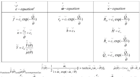
In EMMI the equations are formulated in a non-dimensional form, and are similarly applicable to rate and temperature-dependent deformation of polycrystalline metals. The specific constitutive relationships of the EMMI model describe the kine-matics of large deformation, the elastic and plastic response of the material as well as damage progression due to void growth, and are
Table 1
Non-dimensional plasticity parameters of EMMI.
aFunctions and are expressed as:
given by the following equations:
(1)
(2)
(3)
(4)
(5)
(6)
(7)
(8)
with
where denotes a corrotational rate typically used to make
the formulation frame indifferent, designates a dimensionless
scalar variable, (bold-faced letter) represents a dimensionless second-rank tensor, and indicates a dimensionless time
deriva-tive. In these equations, are the total stress tensor and
its hydrostatic part (pressure); are the total,
elas-tic, and plastic rate of deformation tensors; are the total
and elastic spin tensors; are the internal state variables
of the model, the first two representing strengths for kinematic (tensor) and isotropic (scalar) hardening, and the last one
denot-ing isotropic damage (void volume fraction); is temperature; is a function describing the thermal expansion characteristics of the material; andFvis a function of the Poisson’s ratio. The sym-bols dev(·), tr(·) and||(·)||denote the deviatoric, trace and norm operators of a second-rank tensor.
The normalized temperature-dependent plasticity parameters
of the model are ( ), and they are
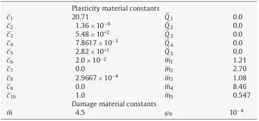
expressed in terms of other constants as given inTable 1. Com-monly, these parameters are used to fit the predicted stress response of the model to experimental stress–strain responses obtained at different temperatures and strain rates. The damage parameters (m,ϕ0), whereϕ0 is the initial void volume fraction,
are usually obtained by fitting the model response to experimental load-displacement data obtained from notched tensile specimen tests. The model has been integrated using a semi-implicit scheme and implemented in commercial finite element codes such as LS-Dyna and ABAQUS (for details, seeMarin et al., 2006).
This plasticity-damage modeling framework described above has experienced success in solving a wide variety of large strain plasticity engineering problems that led to ductile fracture.
Horstemeyer (1992)ran large scale, complex finite element sim-ulations using the model to show the damage progression and final fracture of submarine hulls.Bammann et al. (1993)used the model to capture high rate fracture of steel materials with dif-ferent geometries.Horstemeyer and Revelli (1996)demonstrated the materials processing history effects on the final fracture of
various high rate conditions. In Horstemeyer (2000) the model
was used for forming limit diagrams of aluminum alloys, which required the damage model to quantify the localization and frac-ture that occurred.Horstemeyer et al. (2003)employed the model to capture the damage progression of magnesium notch specimens under different stress triaxialities. Fang et al. (2005)employed the plasticity-damage model to run large scale finite element
simulations of car crashes. Guo et al. (2005) showed how the
experimen-Fig. 3.Experimental and averaged stress–strain responses from copper tensile tests.
tal data, for a variety metal alloys (steel, aluminum, and titanium).
Anurag et al. (2009)applied the model to metal cutting of steel alloys showing that the model captures the nuances of the differ-ent stress states (compression, tension, and torsion) on fracture. The plasticity-damage model, however, has not been used to model the hydroforming process until now.
For the present work, the constants for the material model have been correlated to the experimental stress–strain responses gener-ated from mechanical characterization studies of the copper tube. Tensile tests were performed on a number of standard dogbone specimens cut from the annealed copper blank (prior to being hydroformed). The tests were carried out at room temperature (25◦C) and at a constant strain rate of 0.001/s.Fig. 3shows the stress–strain responses obtained from eight tensile tests. Also pre-sented inFig. 3is the calibrated stress–strain curve from EMMI. Calibration is performed using amatlabcode developed for such purpose (Marin et al., 2006). As the material experiences a range of strain rates during the hydrofoming process, the material model should be able to capture the material’s strain rate dependence. One main parameter of the model that determines the rate sensitivity at room temperature is the exponentn. In this work, its value has been estimated from data published byDao et al. (2007)who reported a rate sensitivity exponent for copper on the order of 1/n≈0.05. As such the bounds fornof 20±15% were used in the calibration routine, giving a computed value ofn=c1+c9/= 20.7,c9= 0 (see Table 2).Fig. 4presents the model correlations computed from
matlab, the experimental stress–strain response, and published stress–strain curves from the literature. The varying strain rate cop-per data shown inFig. 4is taken fromTanner et al. (1999)and
Molinari and Ravichandran (2005), where they have used Oxygen Free High Conductivity (OFHC) copper, a material whose chemi-cal composition is similar to DHP copper. Note the consistency of
Table 2
DHP copper material constants of EMMI.
Plasticity material constants
Fig. 4.Strain rate effects on the stress–strain response of copper.
our experimental data with the literature data. Finally, the damage constants are calibrated using the load-displacement curve for a selected uniaxial tensile test in order to capture the failure strain during tensile loading. This calibration is performed using finite elements due to the non-homogeneous deformation of the speci-men after maximum loading. Results of this fitting procedure are presented inFig. 5. A summary of the EMMI material constants for DHP copper is given inTable 2. Note that most of the temperature-related constants have been set to zero as the experimental data available is limited to one testing temperature (room temperature). During hydroforming, a material point is typically subjected to multi-axial stress states but a biaxial state of stress usually pre-dominates. Hence, hydroforming has been analyzed in the context of tube bulge tests.Fuchizawa and Narazaki (1993)was one of the first to show that a biaxial stress state was more compliant than the response under uniaxial loading.Koc et al. (2001)developed a methodology which can be used to obtain the flow stress curve of tubular materials using on line automated hydraulic bulge tests.
Strano et al. (2004)developed an inverse energy approach to deter-mine the flow stress of tubular materials from the bulge test based
Fig. 5.Fitting the damage parameters (ϕ0= Phio,m= DMR) of EMMI: (a) finite
on an energy balance.Hwang and Lin (2002)developed an ana-lytical relationship investigating the relationship between bulge height and internal pressure for bulge forming.Sokolowski et al. (2000)coupled a hydraulic bulging tool set with Finite Element simulations to determine the proper flow stress of tubular materi-als.Horstemeyer (2000)showed that these multi-axial stress states can be captured by the proposed internal state variable modeling methodology as demonstrated by forming limit diagrams.
3.2. Finite element mesh
The hydroforming process was carried out using six separate components but the mesh comprised only four parts as illustrated inFig. 6: die, bucking plate, ram, and copper billet. The entire finite element model contains 3349 elements chosen from the ABAQUS element library and distributed as follows: 1536 C3D8R (brick) ele-ments for the copper billet, 21 ARSR rigid eleele-ments for the buckling plate, 330 R3D4 elements for the ram, and 1462 R3D4 elements for the die. The deformation of the blank was symmetric along two axes, so a quarter model mesh was implemented to speed up com-putational times.Fig. 7shows that this quarter model only involves one ram, a quarter of the blank, and top and bottom dies. Part geom-etry for the hydroforming dies was imported into ABAQUS CAE as a rigid solid. The hydroforming rams were modeled in ABAQUS as cylindrical rigid shells. The bucking system was modeled as a rigid plate the size of the tee branch cavity in the dies. The dies, rams and bucking system were assumed to be rigid, because of their tool steel composition, which is much harder/stronger than the copper blank.
Fig. 6.The finite element simulation set-up showing the different components of hydroforming process.
3.3. Boundary conditions
The hydroforming process was controlled by a ram
velocity–time history and a pressure–time history curve (see
Fig. 1) and was broken into four steps for the finite element simulations. The pressure–time history controlled the magnitude of the whitewater pressure within the copper blank during the hydroforming process. A more detailed description of the pressure-and velocity–time histories used for the process is shown inFig. 8
along with the finite element steps employed for the boundary
Fig. 8.Simulation steps on pressure–time and velocity–time histories.
conditions (seeFig. 7). The pressure–time history comprised three stages: sealing, forming, and coining. The ram velocity–time his-tory comprised two stages: sealing and forming. The sealing stage for both time histories coincided and the ram forming portion overlapped the forming and coining portions of the pressure–time
histories. During the sealing stage, the ram entered into the tube to seal the end of the copper blank. Once the ram sealed the copper blank, the pressure was initiated to reach the set sealing pressure. During the forming stage, the ram moved slower as the pressure grew to the full forming pressure and the branch of the tee formed. The tee branch formed upward until it pressed the bucking plate to within 0.010 in. (.254 mm) of the hard stop. At this time, the pressure entered the coining stage, ramping to approximately 75 MPa and causing the tee branch to form into all the corners of the die.
The pressure–time history was generated based upon six parameters: maximum sealing pressure, sealing pressure ramp time, maximum forming pressure, forming pressure ramp time, coining pressure, and coining pressure ramp time. The pressure increased from its current value to the set value over the ramp time by following an S-curve. The S-curve was created by fitting a sine wave over the acceleration and deceleration portions of a constant acceleration trapezoidal curve, as shown inFig. 8. Once the pres-sure curve ramped to the desired prespres-sure, a constant prespres-sure was maintained until the next stage of the forming process was reached. The ram velocity–time history displayed inFig. 8was gener-ated based on six parameters: sealing acceleration distance, sealing maximum velocity, sealing travel, forming acceleration distance, forming maximum velocity, and forming travel. The ram veloc-ity increased from zero to the specified velocveloc-ity over the specified
Fig. 10.The effective plastic strain is shown in the color contour for different simulations with the forming pressure decreasing for each simulation. The inset pressure–time history plots illustrate the different simulations with six different pressure histories. Clearly, the higher the gradient between 2 and 4 s yields greater plastic strains.
acceleration distance by following an S-curve similar to the pres-sure curve. The ram S-curve was also a sine wave fit over a constant acceleration trapezoidal curve. Once the ram velocity curve accel-erated to the specified velocity, a constant velocity was maintained until the deceleration portion of the curve was reached. The total ram travel distance was equal to the area under the ram veloc-ity curve. The control system (physical and simulated) calculated the area under the velocity–time history curve. If this area was less than the total travel distance, a constant velocity was added to the ram velocity–time history to reach the specified travel dis-tance. If this area was more than the total travel distance, the acceleration distance was reassigned to half the total travel dis-tance and the maximum velocity was reassigned to the velocity which would have been reached using the original acceleration distance.
Now that the ram movements have been discussed, assump-tions related to the other components will be explained. The die was fixed in such a manner that no displacements or rotations were admitted in any direction. The bucking plate was force controlled as it was designed to inhibit the branch of the tee so fracture would
not occur. The bucking plate was able to move as close as 1.524 mm from the outer diameter of the copper billet. Master-slave surface contacts existed between the copper blank and the die, ram, and bucking plate.
3.4. Preliminary simulation results
Fig. 9shows snapshots at different times of the von Mises stress in the deforming copper blank during the hydroforming simulation. These results were obtained using EMMI without damage (ϕ0= 0). These snapshots depict the connection between the pressure- and velocity–time histories with the stress contours and deforming geometry of the tube throughout the forming process. Clearly, the developed finite element model and corresponding solution pro-cedure with four different steps (seeFig. 7) made the numerical simulation very robust, capturing well the details of the hydroform-ing process.
Fig. 11.The damage level is shown in the color contour for different simulations with the forming pressure decreasing for each simulation. The inset pressure–time history plots illustrate the different simulations with six different pressure histories. Clearly, the higher pressure gradient between 2 and 4 s yields greater damage. Note the apparent volume increase of the elements with high levels of damage (porosity). High values of damage strongly affect the deformation patterns of the hydroformed tube.
pressure (pressure gradient) was varied from approximately 2 to 6 s. Again, this study was performed with EMMI without damage. The results from these simulations are presented inFig. 10, where contour plots of the effective plastic strains at the end of the pro-cess are given. Two observations are important from this figure. First, extremely large strains occur when the pressure gradient is high. Simulations 1–3 all show effective strains up to 500%. Sec-ond, wrinkling (instability from localized buckling) starts to occur as the forming pressure is decreased. Simulation 6 shows the wrin-kling starting in the radius of the tee. On the other hand, simulation 4 and 5 indicates that the pressure gradients used for these cases are adequate to form the tee branch, although simulation 5 uses a lower forming pressure. This numerical study illustrates the fact
that there exists a window of optimum processing parameters that produces well-processed tee-tubes.
Another group of simulations with identical boundary condi-tions as those described above was performed using the EMMI model with damage. The initial value of damage was set to
Fig. 12.Comparison of the finite element simulation results with the experimental results from a well-processed hydroformed tee-tube.
align with the extremely large strains exhibited in Fig. 10. It is important to point out here that, as the hydroforming process is a pressure-driven process, one may expect that the tube blank will experience high stress triaxialities (ratio of the hydrostatic stress to von Mises equivalent stress) in zones with high tensile hydro-static stresses. In fact, the simulations showed maximum stress triaxiality values ranging from 1.3 to 6, depending on the bound-ary conditions. Since the void growth rule used by EMMI depends exponentially on this quantity, high void growth rates are expected to happen for hydroforming boundary conditions inducing large tensile stresses. This behavior has been observed in the numerical simulations.
The above simulations evaluated the robustness of the finite ele-ment model constructed as well as the general capability of the
Fig. 13.Comparison of finite element simulation results with the experimental results from a processed hydroformed tee-tube that induced wrinkling.
EMMI model to predict the large plastic deformations and ductile damage evolution during the hydroforming process. As validation experiments for the damage aspects of the hydrofoming process is lacking (effect of processing parameters on the failure/fracture of copper tee-tubes), the next section of the paper mainly focuses on validating both the process model and the plasticity aspects of EMMI with specific experimental data collected during the study.
4. Simulation/validation results and discussion
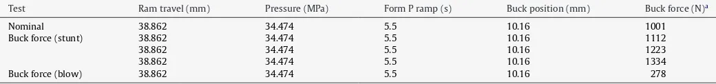
Once the aforementioned hydroforming simulations were per-formed, an experimental validation study was conducted at a hydroforming plant. One check was to compare the material flow patterns of points in the copper blank with that obtained from the numerical simulations. In the plant, the forming pro-cess was set by five main parameters: ram forming travel, forming
Table 3
Validation experiments for hydroforming simulation.
Test Ram travel (mm) Pressure (MPa) Form P ramp (s) Buck position (mm) Buck force (N)a
Nominal 38.862 34.474 5.5 10.16 1001
Buck force (stunt) 38.862 34.474 5.5 10.16 1112
38.862 34.474 5.5 10.16 1223
38.862 34.474 5.5 10.16 1334
Buck force (blow) 38.862 34.474 5.5 10.16 278
Fig. 14.Comparison of material point profiles for the hydroforming validation experiments and the associated numerical simulation results with a varying fric-tion coefficient. Note that when the coefficient of fricfric-tion was= 0.075 the results compared extremely well.
pressure, forming pressure ramp time, bucking punch position, and bucking punch force. For the validation study, some of these parameters were varied in the physical process as
pre-sented by Table 3. Fig. 12 shows clearly that the numerical
predictions compared well with the experimental results for a well-processed tee-tube.Fig. 13 also shows a great comparison of the simulation results with the experiment for a wrinkled tee-tube.
For the simulations related to each set of conditions presented inTable 3, the physical profile of the tubes were measured and compared to the simulation profiles. A simulation of the nom-inal case was used to estimate the friction coefficient for the
hydroforming process using a methodology similar to Ngaile et
al. (2004).Fig. 14presents the physical and simulation profiles of the overall tee and the bottom section of the tee for the nominal case. The comparison shows that the friction coefficient providing the best behavior had a value of= 0.075. This value corrobo-rates results found in Ngaile et al. (2004). The small difference in the bottom wall thickness is probably due to alignment and tolerance issues in the hydroforming tooling. Using the coeffi-cient of friction of 0.075, Fig. 15 shows that the overall and bottom profile for each case included in the validation experi-ments agrees well with those obtained from the hydroforming experiments.
Fig. 15.Comparison of material point profiles for the hydroforming validation experiments and the associated numerical simulation results with a bucking resis-tance. Note that all cases compare very well.
5. Conclusions
A modeling-experimental study was performed on a complex hydroforming process using a non-dimensionalized internal state variable history model (EMMI) that captures strain rate and multi-axial stress state effects. The model constants were determined from uniaxial stress–strain responses and the predictive model was used to evaluate different processing histories. The model was vali-dated from experimental results obtained from in-plant processes. The excellent comparisons indicate that the model can be used to optimize the process space to eliminate wrinkling or fracture. The developed model is used in a second article to perform a parametric study of the copper T-shape tube hydroforming process.
Acknowledgement
This work was performed under the auspices of the Center for Advanced Vehicular Systems (CAVS) at Missisissippi State Univer-sity.
References
Abrantes, J.P., Szabo-Ponce, A., Batalha, G.F., 2005. Experimental and numerical sim-ulation of tube hydroforming (THF). Journal of Materials Processing Technology 164–165, 1140–1147.
Anurag, S., Guo, Y.B., Horstemeyer, M.F., 2009. The effect of materials testing modes on finite element simulation of hard machining via the use of internal state variable plasticity model coupled with experimental study. Computers and Structures 87 (5–6), 303–317.
Bammann, D.J., 1984. An internal variable model of viscoplasticity. In: Aifantis, E.C., Davison, L. (Eds.), Media with Microstructures and Wage Propagation, Interna-tional Journal of Engineering Science, vols. 8–10. Pergamon Press, p. 1041. Bammann, D.J., 1990 May. Modeling temperature and strain rate dependent large
of metals. Applied Mechanics Reviews 43 (5 (Part 2)).
Bammann, D.J., Aifantis, E.C., 1987. Model for finite deformation plasticity. Acta Mechanica 69 (1–4), 97–117.
Bammann, D.J., Chiesa, M.L., Horstemeyer, M.F., Weingarten, L.I., 1993. In: Wierzbicki, T., Jones, N. (Eds.), Failure in Ductile Materials Using Finite Element Methods Structural Crashworthiness and Failure. Elsevier Applied Science, The Universities Press (Belfast) Ltd..
Butcher, C., Chen, Z., Bardelcik, A., Worswick, M., 2009. Damage-based finite-element modeling of tube hydroforming. International Journal of Fracture 155 (1), 55–65. Carrado, A, Duriez, D., Barrallier, L., Bruck, S., Fabre, A., Stuhr, U., Pirling, T., Klosek, V., Palkowski, H., 2008. Variation of Residual Stresses in Drawn Copper Tubes. Trans Tech Publications Ltd., Vienna, Austria, pp. 21–26.
Chen, J.Y., Xia, Z.C., Tang, S.C., 2000. Corner fill modeling of tube hydroforming. Amer-ican Society of Mechanical Engineers, Manufacturing Engineering Division, MED 11, 635–640.
Cherouat, A., Saanouni, K., Hammi, Y., 2002. Numerical improvement of thin tubes hydroforming with respect to ductile damage. International Journal of Mechan-ical Sciences 44 (12), 2427–2446.
Chu, E., Xu, Y., 2004. Hydroforming of aluminum extrusion tubes for automotive applications. Part I. Buckling, wrinkling and bursting analyses of aluminum tubes. International Journal of Mechanical Sciences 46 (2), 263–283. Cocks, A., Ashby, M., 1980. Intergranular fracture during power-law creep under
multiaxial stresses. Metal Science 14, 7.
Daly, D, Duroux, P., Rachik, M., Roelandt, J.M., Wilsius, J., 2007. Modelling of the post-localization behaviour in tube hydroforming of low carbon steel. Journal of Materials Processing Technology 182 (1–3), 248–256.
Dao, M., Lu, L., Asaro, R.J., De Hosson, J.T.M., Ma, E., 2007. Toward a quantitative understanding of mechanical behavior of nanocrystalline metals. Acta Materi-alia 55 (12), 4041–4065.
Fang, H., Solanki, K., Horstemeyer, M.F., 2005. Numerical simulations of multiple vehicle crashes and multidisciplinary crashworthiness optimization. Interna-tional Journal of Crashworthiness 10 (2), 161–171.
Frost, H., Ashby, M., 1982. Deformation Mechanism Maps. Pergamon Press. Fuchizawa, S., Narazaki, M., 1993. Bulge test for determining stress–strain
charac-teristics of thin tubes. Advanced Technology of Plasticity, 6.
Grey, J.E., Deveraux, A.P., Parker, W.N., 1939. Apparatus for Making Wrought Metal T’s.
Guan, Y., Pourboghat, F., Barlat, F., 2006. Finite element modeling of tube hydro-forming of polycrystalline aluminum alloy extrusions. International Journal of Plasticity 22 (12), 2366–2393.
Guo, Y.B., Wen, Q., Horstemeyer, M.F., 2005. An internal state variable plasticity-based approach to determine dynamic loading history effects on material property in manufacturing processes. International Journal of Mechanical Sci-ences 47, 1423–1441.
Hama, T., Asakawa, M., Fuchizawa, S., Makinouchi, A., 2003. Analysis of hydrostatic tube bulging with cylindrical die using static explicit FEM. Materials Transac-tions 44 (5), 940–945.
Heo, S.C, Kim, J., Kang, B.S., 2006. Investigation on determination of loading path to enhance formability in tube hydroforming process using APDL. Journal of Materials Processing Technology 177 (1–3), 653–657.
Horstemeyer, M.F., 1992. Damage of HY100 steel plates from oblique constrained blast waves. In: Giovanola, J.H., Rosakis, A.J. (Eds.), Advances in Local Frac-ture/Damage Models for the Analysis of Engineering Problems, vol. 137. ASME AMD, Book No. H00741.
Horstemeyer, M.F., 2000. A numerical parametric investigation of localization and forming limits. International Journal of Damage Mechanics 9, 255–285. Horstemeyer, M.F., Revelli, V., 1996. Stress history dependent localization and
fail-ure using continuum damage mechanics concepts. In: McDowell, D.L. (Ed.), Application of Continuum Damage Mechanics to Fatigue and Fracture. ASTM, STP1315.
Horstemeyer, M.F., Wang, P., 2003. Cradle-to-grave simulation-based design incorporating multiscale microstructure–property modeling: reinvigorating design with science. Journal of Computer-Aided Materials Design 10, 13–34.
Horstemeyer, M.F., Lathrop, J., Gokhale, A.M., Dighe, M., 2000. Modeling stress state dependent damage evolution in a cast Al–Si–Mg aluminum alloy. Theoretical and Applied Fracture Mechanics 33, 31–47.
Horstemeyer, M.F., Gall, K.A., Dolan, K., Haskins, J., Gokhale, A.M., Dighe, M.D., 2003. Numerical, experimental, and image analyses of damage progression in cast A356 aluminum notch tensile bars. Theoretical and Applied Fracture Mechanics 39 (1), 23s–45s.
Hwang, Y.-M, Lin, Y.-K., 2002. Analysis and finite element simulation of the tube bulge hydroforming process. Journal of Materials Processing Technology (125), 4.
Islam, M.D., Olabi, A.G., Hashmi, M.S.J., 2006. Feasibility of multi-layered tubular components forming by hydroforming and finite element simulation. Journal of Materials Processing Technology 174 (1–3), 394–398.
Islam, M.D, Olabi, A.G., Hashmi, M.S.J., 2008. Mechanical stresses in the multilayered T-branch hydroforming: numerical simulation. International Journal of Manu-facturing Technology and Management 15 (2), 238–245.
Jansson, M., Nilsson, L., Simonsson, K., 2005. On constitutive modeling of aluminum alloys for tube hydroforming applications. International Journal of Plasticity 21 (5), 1041–1058.
Jirathearanat, S, Hartl, C., Altan, T., 2004. Hydroforming of Y-shapes—product and process design using FEA simulation and experiments. Journal of Materials Pro-cessing Technology 146 (1), 124–129.
Kashani Zadeh, H., Mashhadi, M.M., 2006. Finite element simulation and experi-ment in tube hydroforming of unequal T shapes. Journal of Materials Processing Technology 177 (1–3), 684–687.
Kim, S.-W., Song, W.-J., Kang, B.-S., Kim, J., 2009. Bursting failure prediction in tube hydroforming using FLSD. International Journal of Advanced Manufacturing Technology 41 (3–4), 311–322.
Koc, M., 2003. Investigation of the effect of loading path and variation in material properties on robustness of the tube hydroforming process. Journal of Materials Processing Technology 133 (3), 276–281.
Koc, M, Altan, T., 2001. An overall review of the tube hydroforming technology. Journal of Materials Processing Technology 108, 9.
Koc, M., Aue-U-Lan, Y., Altan, T., 2001. On the characteristics of tubular materials for hydroforming experimentation and analysis. International Journal of Machine Tools & Manufacture 41, 11.
Kocanda, A, Sadlowska, H., 2006. An approach to process limitations in hydroforming of X-joints as based on formability evaluation. Journal of Materials Processing Technology 177 (1–3), 663–667.
Kulkarni, A., Biswas, P., Narasimhan, R., Luo, A.A., Mishra, R.K., Stoughton, T.B., Sachdev, A.K., 2004. An experimental and numerical study of necking initia-tion in aluminium alloy tubes during hydroforming. Internainitia-tional Journal of Mechanical Sciences 46 (12), 1727–1746.
Marin, E.B, Bammann, D.J., Regueiro, R.A., Johnson, G.C., 2006. On the Formula-tion, Parameter Identification and Numerical Integration of the EMMI Model: Plasticity and Isotropic Damage. Sandia National Laboratories, pp. 94. Mohammadi, Mosavi Mashadi (2009) determined the proper loading paths via FEM
and a fuzzy controller.
Molinari, A., Ravichandran, G., 2005. Constitutive modeling of high-strain-rate defor-mation in metals based on the evolution of an effective microstructural length. Mechanics of Materials, 37.
Ngaile, G., Jaegar, S., Altan, T., 2004. Lubrication in tube hydroforming. Part II. Perfor-mance evaluation of lubricants using LDH test and pear-shaped tube expansion test. Journal of Materials Processing Technology 146, 7.
Shirayori, A., Fuchizawa, S., Narazaki, M., 2002. Influence of Initial Thickness Devi-ation in Tube Periphery on Tube DeformDevi-ation During Free Hydraulic Bulging. Society of Manufacturing Engineers, West Lafayette, ID, United States, p. 1–8. Shirayori, A., Fuchizawa, S., Narazaki, M., 2004. A Design Method of Loading Paths for
Tube Hydroforming Using FEM Simulator. Society of Manufacturing Engineers, Charlotte, NC, United States, pp. 629–636.
Smith, L.M., Ganeshmurthy, N., Murty, P., Chen, C.C., Lim, T., 2004. Finite element modeling of the tubular hydroforming process. Part 1. Strain rate-independent material model assumption. Journal of Materials Processing Technology 147 (1), 121–130.
Sokolowski, K., Gerke, M., Ahmetoglu, M., Altan, T., 2000. Evaluation of tube forma-bility and material characteristics: hydraulic bulge testing of tubes. Journal of Materials Processing Technology 98, 6.
Strano, M., Jirathearanat, S., Shiuan-Guang Shr, Altan, T., 2004. Virtual process devel-opment in tube hydroforming. Journal of Materials Processing Technology (146), 6.
Strano, M., Jirathearanat, S., Altan, T., 2001. Adaptive fem simulation for tube hydroforming: a geometry-based approach for wrinkle detection. CIRP Annals—Manufacturing Technology 50 (1), 185–190.
Tanner, A.B., McGinty, R.D., McDowell, D.L., 1999. Modeling temperature and strain rate history effects in OFHC Cu. International Journal of Plasticity, 15. Varma, N.S.P, Narasimhan, R., Luo, A.A., Sachdev, A.K., 2007. An analysis of