Full Terms & Conditions of access and use can be found at
http://www.tandfonline.com/action/journalInformation?journalCode=ubes20
Download by: [Universitas Maritim Raja Ali Haji] Date: 11 January 2016, At: 19:39
Journal of Business & Economic Statistics
ISSN: 0735-0015 (Print) 1537-2707 (Online) Journal homepage: http://www.tandfonline.com/loi/ubes20
Sparse and Stable Portfolio Selection With
Parameter Uncertainty
Jiahan Li
To cite this article: Jiahan Li (2015) Sparse and Stable Portfolio Selection With
Parameter Uncertainty, Journal of Business & Economic Statistics, 33:3, 381-392, DOI: 10.1080/07350015.2014.954708
To link to this article: http://dx.doi.org/10.1080/07350015.2014.954708
Accepted author version posted online: 21 Aug 2014.
Submit your article to this journal
Article views: 248
View related articles
View Crossmark data
Sparse and Stable Portfolio Selection With
Parameter Uncertainty
Jiahan L
IDepartment of Applied and Computational Mathematics and Statistics, 156 Hurley Hall, University of Notre Dame, Notre Dame, IN 46556 ([email protected])
A number of alternative mean-variance portfolio strategies have been recently proposed to improve the empirical performance of the classic Markowitz mean-variance framework. Designed as remedies for parameter uncertainty and estimation errors in portfolio selection problems, these alternative portfolio strategies deliver substantially better out-of-sample performance. In this article, we first show how to solve a general portfolio selection problem in a linear regression framework. Then we propose to reduce the estimation risk of expected returns and the variance-covariance matrix of asset returns by imposing additional constraints on the portfolio weights. With results from linear regression models, we show that portfolio weights derived from new approaches enjoy two favorable properties: sparsity and stability. Moreover, we present insights into these new approaches as well as their connections to alternative strategies in literature. Four empirical studies show that the proposed strategies have better out-of-sample performance and lower turnover than many other strategies, especially when the estimation risk is large.
KEY WORDS: Mean-variance analysis; Penalized least squares; Portfolio selection; Shrinkage estimation.
1. INTRODUCTION
Expected returns and covariance matrix are two inputs of a portfolio selection problem. If the true expected returns and true covariance matrix are known to investors, mean-variance analysis guarantees the optimal portfolio positions. However, since these two parameters have to be estimated from historical data, the out-of-sample performance of mean-variance analysis is impacted by parameter uncertainty and estimation errors. In portfolio management literature, it has long been recognized that the sample mean and the sample covariance matrix are suboptimal, and usually deliver extremely poor out-of-sample performance (for a review, see Brandt2009).
To reduce the undesired impact of sample estimates, shrink-age estimators of expected returns and covariance matrix were proposed (Jorion 1986; Ledoit and Wolf 2003; 2004). Alter-natively, methods have been proposed to directly address the decision variable of a portfolio selection problem: the port-folio weights. These methods solve the classic problem with sample mean and sample covariance matrix, but impose ad-ditional constraints on the portfolio weights. Jagannathan and Ma (2003) studied the shortsale-constrained global minimum-variance portfolio. They found that such constraints actually im-prove the empirical performance of portfolios. DeMiguel et al. (2009) and Brodie et al. (2009) proposed the global minimum variance portfolio with the L1-norm constraint or the L2-norm constraints on the portfolio weights. Behr, Guettler, and Miebs (2013) imposed flexible upper and lower bounds on each portfo-lio weight, allowing their strategy to nest different benchmarks. All the above portfolio strategies constrain the magnitude of portfolio weights in different ways. These constraints generate suboptimal solutions if true parameters are known, but may be beneficial in the presence of parameter uncertainty and estima-tion risk. Since extreme portfolio weights are usually brought by large estimation errors of unknown parameters rather than true parameter values of the population, correcting the portfolio
weights directly amounts to reducing the impact of parame-ter uncertainty (Frost and Savarino1986; Jagannathan and Ma
2003; Garlappi, Uppal, and Wang2007).
In this article, we first show how a general portfolio selection problem can be recast as a regression problem, so that esti-mating portfolio weights is equivalent to estiesti-mating regression coefficients in a linear regression model. Britten-Jones (1999) proposed the regression formulation of a tangency portfolio, and Fan, Zhang, and Yu (2012) showed how Markowitz’s risk min-imization problem can be formulated as a regression problem. However, no regression formulation was proposed for a general mean-variance portfolio selection problem. The first part of this article will fill this gap, allowing the existing statistical theory of regressions to provide valuable insights into portfolio selection problems. For our problem in particular, this framework implies that imposing additional constraints on the portfolio weights is equivalent to imposing additional constraints on regression coefficients.
We then study the weight-constrained mean-variance portfo-lios. Shrinking portfolio weights directly makes sense for three reasons. First, Fan, Zhang, and Yu (2012) showed that the esti-mation risk is bounded by a quadratic function of the L1 norm of portfolio weights, and thus constraining portfolio norms is equivalent to constraining estimation risks. Second, estimation errors may accumulate through arithmetic operations in calcu-lating portfolio weights. By working on the portfolio weights directly, their desired forms and properties could be achieved. Moreover, the magnitude of portfolio weights is a proxy for the transaction cost (e.g., Brodie et al.2009).
© 2015American Statistical Association Journal of Business & Economic Statistics
July 2015, Vol. 33, No. 3 DOI:10.1080/07350015.2014.954708
Color versions of one or more of the figures in the article can be found online atwww.tandfonline.com/r/jbes.
381
We further propose two favorable properties of portfolio weights when the number of assets is large: sparsity and sta-bility, and show how constraints could encourage these two properties. With sparsity, portfolio weights could be zero for a subset of assets. In fact the idea of sparsity has been implicitly explored. If a portfolio selection procedure predetermines a sub-set of candidate assub-sets, the resulting portfolio is sparse, since it effectively assigns zero weights to the rest of the assets. Sparse portfolio strategies are also those who test the hypothesis that whether some small portfolio weights are not significantly dif-ferent from zero. If the data suggest that some portfolio weights are not statistically different from zero, setting them to zero re-duces portfolio variance and ameliorate the impact of parameter uncertainty (Britten-Jones, 1999; Garlappi, Uppal, and Wang
2007).
Other than sparsity, portfolio stability is another desirable property, since in practice, extremely variable positions are usu-ally observed from the classic mean-variance framework. Such instability is largely due to the estimation errors in the esti-mated covariance matrix as well as the step of taking its inverse. As a result, large positions lead to abysmal out-of-sample per-formance rather than efficient diversification. Given these two favorable properties of portfolio rules, we will demonstrate how the new approaches address these issues directly. We estimate the sparse and stable portfolio weights in the framework of penalized least squares. Intuitively if all excess returns are un-correlated and have a common variance, the new approach is equivalent to shifting and scaling the portfolio weights derived from the sample estimates toward zero. In this way, small port-folio weights are set to zero, and extremely large positions are regulated, resulting in sparse and stable portfolios.
Finally we examine the relation between our new approaches and various robust portfolio selection approaches in literature, including the portfolio using the empirical Bayes-Stein estima-tors (Jorion 1986), the ambiguity averse portfolio (Garlappi, Uppal, and Wang2007), and those based on the shrinkage es-timators of covariance matrix (Ledoit and Wolf 2003; 2004). Interestingly, although many other portfolio rules start with dif-ferent assumptions and considerations, the proposed framework nests them as special cases with different levels of sparsity or stability. Empirical analyses suggest that the portfolio strategies developed in this article have superior out-of-sample perfor-mance with relatively low turnover. The conclusion is stronger if parameter uncertainty is larger.
The rest of this article is organized as follows. Section 2
presents the regression formulation of portfolio selection prob-lems. Section3proposes four weight-constrained portfolios, and shows how sparse and stable portfolio weights are achieved. In Section4, the connections between new strategies and other ro-bust portfolio strategies are discussed. Section5presents meth-ods for and results from empirical studies. In Section 6, we provide concluding remarks.
2. REGRESSION APPROACH FOR SHRINKAGE
ESTIMATIONS
Consider a standard portfolio choice problem withNrisky as-sets. Suppose the excess returns at timet,Rt, follow a
multivari-ate normal distribution with mean µand variance-covariance
matrix, whereµis anN×1 vector,is anN×N matrix andRt is the asset returns in excess of risk-free rate. At timet
an investor determines the portfolio weightswto maximize the mean-variance objective function:
U(w)=wTµ−γ 2w
T
w, (1)
whereγ >0 is the coefficient of relative risk aversion. The op-timal portfolio weights are given byw= γ1−1µ. Proposition 1 shows that the portfolio choice problem can be formulated as a linear regression problem.
Proposition 1. Consider the following multiple linear regres-sion withNindependent variables andNobservations:
y=Xw+e, (2)
whereyis anN-dimensional dependent variable,Xis anN×N
matrix of independent variables,wis anN-dimensional vector
of regression coefficients, andeis a vector of random errors.
Let
X=√γ 12 (3)
and
y= √1
γ
−12µ. (4)
Then the least squares estimator ofw, ˆwOLS=(XTX)−1(XTy),
is the same as the optimal portfolio weights ˆw= 1γ−1µ. In
other words, the least squares estimator solves the portfolio selection problem (1).
Since both µ and are unknown to investors, in practice plug-in strategy is a popular one (Kan and Zhou2007; Brandt
2009). This two-step strategy first replaces both unknown pa-rameters in (1) or equivalently (3)–(4) by their estimates based on historical data. Then optimization is carried out to find out the optimal portfolio weights conditional on the estimated parame-ters. Among all estimators, the maximum likelihood estimators
ˆ
µand ˆare widely used, where ˆµ=. . .(Rt−µˆ)T, withT
be-ing the total number of observations. Then the optimal portfolio maximizes
U(w)=wTµˆ −γ 2w
Tw.ˆ (5)
This plug-in strategy is intuitive and convenient, but fails to take into account parameter uncertainty and estimation risk. There are three sources of estimation errors: estimated mean ˆµ, estimated covariance matrix ˆ, and the inverse operator on the estimated covariance matrix. In fact, when two return series are highly correlated, the estimation error in ˆcould be amplified dramatically by the inverse operator, resulting in highly volatile
ˆ
−1 and ˆw. One advantage of linear regression formulation is to test the estimator ˆw formally using statistical inference procedures. For example, by solving for the tangency portfo-lio using a regression approach, Britten-Jones (1999) provided estimates of the portfolio weights and the associated standard errors, and tested the hypothesis that some weights are zero. Similar approaches for constructing confidence intervals and testing hypothesis can also be formulated under our linear re-gression approach for portfolio selections.
3. A GENERAL FRAMEWORK
In this section, we propose four portfolio strategies that solve the standard problem subject to additional constraints on the portfolio weights. Portfolio rules associated with these strategies can be regarded as shrinkage estimators of portfolio weights.
3.1 Sparse Portfolio
When a subset of assets receives zero weights, the portfolio rule is said to be sparse. Sparse portfolio weights have been im-plicitly explored in the finance literature. Britten-Jones (1999) proposed t-test and F-test for testing whether the estimated weight for an asset or a group of assets is statistically differ-ent from zero. The test provides direct guidance in constructing efficient portfolios and assessing the estimation risk. Garlappi, Uppal, and Wang (2007) provided a solution for a portfolio se-lection problem that explicitly considers parameter uncertainty. They suggested (in their Proposition 3) that an investor should set the portfolio weights to zero and invest only in risk-free as-set if the estimated squared Sharpe ratio, ˆθ2=µˆTˆ−1µˆ, is not
statistically different from zero. This hypothesis upon which in-vestment decisions are based is easy to test, since the sampling distribution of ˆθ2is a scaled F-distribution, or ˆθ2∼ TN
−NFN,T−N
(Kan and Zhou2007).
When the number of assets is large, sparse portfolio rule is de-sired. First of all, zero portfolio weights reduce transaction cost as well as portfolio management cost. Second, since the number of historical asset returnsT is relatively small compared with the number of assetsN, estimation error is large. By setting a subset of small portfolio weights to zero, the estimated portfolio weights are no longer unbiased, but their variances and the mean squared prediction errors could be reduced. This is also known as bias-variance tradeoff.
Sparse portfolio weights can be obtained by constraining the L1 norm of portfolio weights. Interestingly, this L1 norm is also related to the upper bound of the estimation risk. Fan, Zhang, and Yu (2012) showed that for the general portfolio choice problem (1),
|U(w; ˆµ,ˆ)−U(w;µ, )| ≤ ||µˆ −µ||∞||w||1
+γ
2||ˆ −||∞||w||
2
1, (6)
whereU(w;θ1, θ2)=wTθ1−γ2wTθ2w,||µˆ −µ||∞and||ˆ −
||∞ are the maximum component-wise estimation error, and
||w||1=Nj=1|wj|is the L1 norm of vectorw. Therefore, as
long as||w||1is bounded, the estimation error is controlled by
the largest component-wise error.
To this end, we propose to estimate the portfolio weights by
Rule I: wˆL1 =argmax
w
wTµˆ −γ 2w
Twˆ ,
subject to ||w||1< s1, (7)
where ˆ and ˆµare maximum likelihood estimates ofandµ respectively, ands1 >0 is a constant. If one letsX=√γˆ
1 2
andy= √1γˆ−12µˆ, the linear regression framework for
portfo-lio selection together with the method of Lagrange multipliers
imply the following:
ˆ
wL1=argmin
w
||y−Xw||22+λ1||w||1
, (8)
whereλ1>0 is a constant, and||.||22is the squared L2 norm of
a vector. This objective function extends ordinary least squares (OLS), and is known as penalized least squares.
When λ1=0, the sizes of |wj|, j =1, . . . , N are not
penalized. When λ1>0, the portfolio weights wˆL1=
( ˆwL1,1, . . . ,wˆL1,N)T are shrunk toward zero in a way that, if
the OLS estimate ˆwj is small enough in absolute value, the
pe-nalized least squares estimate ˆwL1,j is exactly zero. Otherwise,
ˆ
wL1,jis ˆwjminus some constant when ˆwj >0, or ˆwj plus some
constant if it is negative (Tibshirani,1996). In other words, with the L1 norm constraint we may have sparse portfolio weights. Such a shrinkage scheme implies that assets receiving small positions may be excluded from the portfolio.
L1 norm penalized regressions have been popular in statis-tics (e.g., Tibshirani1996) and econometrics (e.g., Bai and Ng
2008; De Mol, Giannone, and Reichlin2008). By recovering the reduced structure in a lower dimensional space, this technique is capable of producing a better estimator of regression coeffi-cient. Although the estimator is biased, it can have substantially lower variance than OLS, leading to a lower mean squared error (MSE). Such reduction of MSE could balance the in-sample performance and the out-of-sample performance of a statistical model.
Note that there is another way of constructing sparse portfo-lio weights, namely hard-thresholding strategy. Using the linear regression formulation without constraints outlined in Section
2, each portfolio weight can be tested with the null hypothesis being that the weight is zero (Britten-Jones1999). Then those assets whose weights are not statistically different from zero are excluded from the portfolio. This strategy, however, tends to be associated with unstable portfolios. To gain more insights, we assume asset returns are uncorrelated, and compare the results of hard-thresholding strategy to those of L1 norm constrained portfolio. For any given assetj,Figure 1plots the classic portfo-lio weight ˆwj, which is thejth element of ˆw= γ1ˆ−1µˆ, versus
the portfolio rule derived from the hard-thresholding strategy (Figure 1(a)) or the rule derived from the L1 norm-constrained strategy (Figure 1(b)). Clearly, both strategies are modifications of ˆwj. However, since estimator ˆwj is a random variable that
changes slightly if new observations are available in estimating µand, the change may result in jumps of portfolio weights from the hard-thresholding strategy. On the other hand, port-folio weights from imposing L1 norm constraint will change continuously, and thus are robust against estimation errors.
3.2 Stable Portfolio
The stability of portfolio weights is another desirable property that has been explicitly explored in literature (Ledoit and Wolf
2003;2004; Brodie et al.2009). It has been documented that in mean-variance efficient portfolios, extreme positions are usually observed, and portfolio weights may change dramatically when new return information is used, as well as when a set of assets becomes unavailable for trading (Garlappi, Uppal, and Wang
2007; Brandt2009). These stylized facts are mainly due to large
Figure 1. Alternative portfolio rules as a function of the portfolio weight derived from the sample mean and the sample covariance matrix. (a) Hard-thresholding portfolio rule. (b) The L1 norm constrained portfolio rule. (c) The portfolio rule that scales the classic portfolio weights by a constant smaller than zero (Ledoit and Wolf2004; Garlappi, Uppal, and Wang2007; Kan and Zhou2007). (d) The portfolio rule with both L1 norm constraint and L2 norm constraint. All excess returns are assumed to be uncorrelated.
estimation errors contained in ˆand the inverse operation on ˆ (Ledoit and Wolf2003). In fact when returns of assetiand assetj
are highly correlated, ˆ−1is highly volatile with extreme entries
(i,i), (i,j), (j,i), and (j,j), resulting in extreme positions in asseti
and assetjthat swing dramatically over time. Hence imposing stability constraints is expected to reduce the estimation risk due to parameter uncertainty and multicollinearity.
Motivated by this observation, improved estimators ofwere proposed. Ledoit and Wolf (2003,2004) proposed the general form of the shrinkage estimator of:
ˆ
s =vˆ +(1−v) ˆg,
where ˆgis a shrinkage target with lower variances, andvis the
shrinkage intensity. Ledoit and Wolf (2003,2004) further de-rived closed-form solutions forv, and demonstrated the superior out-of-sample performance of this strategy. We show in the next proposition that replacing ˆwith ˆsin (5) is equivalent to
im-posing a constraint on a quadratic form of the portfolio weight, and how its solution is connected with the classic solution ˆw.
Proposition 2. The optimal mean-variance portfolio
selec-tion problem with a shrinkage estimator of covariance matrix ˆ
s =vˆ +(1−v) ˆg
ˆ
w=argmax w
wTµˆ −γ 2w
Tˆ sw
(9)
is equivalent to the problem
ˆ
w=argmax w
wTµˆ0−
γ 2w
Twˆ subject to wTˆ gw < s,
(10) where ˆµ0= µvˆ, andsis a positive constant inversely proportional
toλ= γ(12−vv) >0. The solution is given by
ˆ w=
I
−A v
ˆ
w, (11)
where matrixA=ˆ−1L(γ C−1+LTˆ−1L)−1LT,Lis a
lower-triangular matrix, and C is a diagonal matrix satisfying the
10
20
30
40
1987 1990 1994 1998 2002 2006 2010 2014
1
1
02
03
04
0
1986 1990 1994 1998 2002 2006 2010 2014
1
1
02
03
04
05
0
(a) (b)
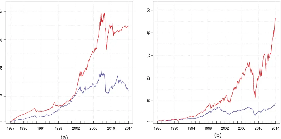
Figure 2. Cumulative wealth of “Rule IV” (red) relative to the benchmark (blue) with initial wealth of$1. (a) Investing in G10 country bonds, (b) investing in 500 individual stocks.
Cholesky decomposition of a positive definite matrix 2λˆg = LCLT.
Therefore, shrinking covariance matrix amounts to taking a linear transformation of the portfolio weight, where the transfor-mation depends on both shrinkage intensityvand the shrinkage target ˆg. When the target covariance matrix is an identity
ma-trix (Ledoit and Wolf2004), it is straightforward to verify that as the covariance matrix is shrunk toward the target,A→I, and the weight is shrunk toward zero. Moreover, when the expected returns are uncorrelated with a lower variance 0< δ2<1, this
strategy is equivalent to scaling the sample portfolio weights ˆw by a constantv+(11+v)δ2 (seeFigure 1(c)).
3.3 Sparse and Stable Portfolio
The above discussion motivates how to achievebothsparsity and stability in a portfolio choice problem. First we could ex-tend the L1 norm constrained portfolio (7) by incorporating a shrinkage estimator ofand propose
ˆ
where ˆMKT is the covariance matrix implied by the
single-factor model (Ledoit and Wolf 2003), ˆCC is a
constant-correlation covariance matrix (Ledoit and Wolf2004),vis the shrinkage intensity, ands1≥0 is a constant. Proposition 2
im-plies that
Other than methods in portfolio management literature, statis-tical methods are also available to stabilize the portfolio weights. It is well-known that if the sample covariance matrix ˆis near singular matrix or ill-conditioned, inverting it is numerically un-stable. Adding a constant along its diagonal fixes the problem, producing a stable estimate of its inverse. This is a standard technique to handle multicollinearity problem in regressions, and is known as ridge regression. Since portfolio weights are linear functions of estimated inverse covariance matrix, this pro-cedure stabilizes the portfolio weights. Specifically, we have
ˆ
where δ >0 is a constant and I is an identity matrix. It is straightforward to show that the problem is equivalent to
Rule IV: wˆL1L2=argmax
L2 norm of a vector.
Whens1=s2= ∞, the portfolio weights derived from (14),
(15), and (17) are unbounded, and the problem reduces to a standard one (5). Whens2= ∞, the problem is the L1 norm
constrained one. When both s1 ands2 are positive, the
port-folio weights are shrunk toward zero in two different ways, promoting both sparsity and stability. In statistics literature, a combination of L1 norm constraint and L2 norm constraint is known as “elastic-net” (Zou and Hastie2005). In a regression problem if theith column and thejth column ofXare highly cor-related and both independent variables are important, regression with only L1 norm constraint tends to assign a large estimate to one of ˆβi and ˆβj randomly, and set the other to zero (Efron
et al. 2004; Zou and Hastie2005). But with an additional L2 norm constraint, regression with both constraints tends to pro-duce similar estimates of ˆβi and ˆβj while maintaining sparsity.
Hence Zou and Hastie (2005) described the combination of L1 constraint and L2 constraint as “a stretchable fishing net that retains all the big fish.”
Note that all objective functions of the proposed portfolio strategies (7), (14), (15), and (17) can be written as a penalized
proaches differ in terms of howXandyare defined, and whether λ2 =0. We determine tuning parameters λ1 andλ2 by
cross-validation (see also DeMiguel et al. 2009) and estimate the penalized least squares with the coordinate descent algorithm.
InFigure 1(d), we visualize the effect of simultaneously im-posing two constraints when the asset returns are uncorrelated. It can be seen that its consequence is a mixture of consequences of imposing L1 norm constraint and L2 norm constraint sepa-rately. That is, ˆw is scaled and then shifted toward zero. The scaling is a consequence of the stabilized problem, while those assets whose weights are small after stabilizing the problem are excluded from the portfolio.
When the portfolios are monthly rebalanced and the number of assets is large, say 500, at least 42 years’ monthly returns are required, so that the sample covariance matrix ˆ is invertible andXandyin (7), (14), (15), and (17) are well-defined. Three
approaches can address this practical issue. First, longer time series of returns could be used to estimate. But other than the data availability issue for most of the securities, such strategy im-poses an unrealistic assumption that the true covariance matrix is time-invariant. The second approach is to estimate this low-frequency covariance matrix by high-low-frequency returns. This strategy gains popularity in recent years due to the availabil-ity of high-frequency financial data (see, e.g., Andersen et al.
2001). However, high-frequency returns from nontraditional as-set classes, such as mutual funds, hedge funds, real asas-sets and
private equity, are generally unavailable. The third approach is to estimate the N-dimensional covariance matrix directly us-ing T < N observations by novel statistical techniques. Fan, Liao, and Mincheva (2013) proposed the principal orthogonal complement thresholding (POET) method for calculating high-dimensional covariance matrices. This method assumes com-mon factors underlying returns, and estimates their covariance matrix by applying thresholding to the part of the sample co-variance matrix that cannot be explained by the factor structure. As a result, the POET estimator is optimization-free and asymp-totically invertible. In what follows, we choose to use the POET estimator ˆPOETwhenN > T.
4. CONNECTIONS TO EXISTING PORTFOLIO
STRATEGIES
4.1 Connection to Plug-in Approaches
The standard solution to the portfolio selection problem ˆw=
1
γˆ−
1µˆ is a plug-in approach where µ and are estimated
by the maximum likelihood estimators (MLEs). Since MLEs are invariant under reparameterization, ˆw is also a maximum likelihood estimator. Kan and Zhou (2007) also considered two other plug-in approaches, which estimateby ¯= TT−1ˆ and
˜ = T T
−N−2ˆ, leading to the unbiased estimators ofandw,
respectively.
Other than three simple plug-in rules, approaches incorporat-ing parameter uncertainty could take similar forms as plug-in approaches. For example, by assuming standard diffusion pri-ors onµand(Klein and Bawa1976; Stambaugh1997), the Bayesian approach is essentially a plug-in rule that estimates
by ˆBayes= T−T+N1−2ˆ. Moreover, Kan and Zhou (2007) derived
the optimal two-fund rule that maximizes the expected out-of-sample performance by estimatingusing ˆtwo−fund=/cˆ 2,
wherec2∈(0,1) is a constant.
Since all these methods scale ˆby a constantcgreater than one, the resulting solution ˆwplug−in is a scaled version of ˆw=
1
γˆ−
1µˆ, or
ˆ
wplug−in=
1
cw.ˆ (19)
This relates ˆwL1L2in rule IV to these plug-in approaches.
How-ever, our approach is more general, in the sense that it determines the scaling factor adaptively from the data and further shifts the scaled portfolio weights to encourage sparsity.
4.2 Connection to the Shrinkage Estimator ofµ
In formulating our portfolio rules, we have shown the effect of replacing ˆwith an shrinkage estimator. Jorion (1986,1991) also proposed a shrinkage estimator ofµ. It shrinks the vector of sample mean ˆµtoward a common target ˆµg, resulting in a
Bayes–Stein estimator
ˆ
µBS=(1−v) ˆµ+vµˆg, with µˆg =
1T Nˆ−1µˆ
1T Nˆ−11N
,
wherev∈(0,1) and the shrinkage target ˆµg is the average
ex-cess return over the risk-free rate of the sample global minimum-variance portfolio.1
Shrinking the sample mean ˆµtoward a target appropriately could reduce the expected quadratic loss of the estimator (Stein
1956; Berger 1985). The following proposition provides the solution to a portfolio selection problem whereµis estimated by ˆµBS, and relates this method to our approach.
Proposition 3. The optimal portfolio choice problem with a
shrinkage estimator of mean ˆµBS=vµˆ+(1−v) ˆµtarget
ˆ
wµ=argmax w
wTµˆBS−
γ 2w
Twˆ (20)
has a solution
ˆ wµ=
1 1+λwˆ +
λ
1+λwˆtarget,
whereλ= 1−vv >0, and ˆwtarget=γ1ˆ−1µˆtargetis the portfolio
weight onceµis estimated by the shrinkage target ˆµtarget.
In particular, when the shrinkage target ˆµtargetis the average
excess return on the sample global minimum-variance portfo-lio 1Nµˆg (Jorion 1986,1991),Nj=1wˆµ,j =Nj=1wˆj. Under
the mild condition||ˆ−1(1
Nµˆg)||1<||ˆ−1µˆ||1, the portfolio
weight is shrunk toward zero, orN
j=1|wˆµ,j|<Nj=1|wˆj|.
Therefore, incorporating the shrinkage estimator ofµis to find a linear combination of sample portfolio weight ˆwand the target portfolio weight ˆwtarget. If the shrinkage target ˆµgequals
zero, the portfolio weight ˆwµ is exactly a scaled version of
ˆ
w, resembling the effect of imposing the L2 norm constraint. Otherwise, the portfolio weight is scaled and shifted, as how the portfolio weights behave once both norm constraints are imposed.
4.3 Connection to Multiprior Approach
Garlappi, Uppal, and Wang (2007) considered the portfolio selection problem that explicitly takes into account parameter uncertainty (or ambiguity) and investors’ aversion to such ambi-guity. They imposed an additional constraint on (5) to reflect the ambiguity aversion (AA), so that the probability of true param-eters being in respective confidence intervals is large. In other words,
P T(T
−N)
(T −1)N( ˆµ−µ)
T−1( ˆµ
−µ)≤ǫ
=1−p, (21)
whereis assumed to be known,ǫis a scalar proportional to the level of ambiguity and ambiguity aversion, andpis a significant level. They showed that when constraint (21) is imposed, the
1Jorion’s approach was motivated from a Bayesian perspective. By assigning an informative conjugate prior for asset returns, empirical Bayes approach suggests that the mean of the predictive density function of asset returns takes the form of ˆµBS=(1−v) ˆµ+vµˆg, where ˆµg“happens to be the average return for the
minimum variance portfolio” (see p. 285 of Jorion1986).
solution is This portfolio rule has an interesting interpretation. Note that
1 2γ( ˆµ
T−1µˆ) is the resulting expected utility once the classic
portfolio rule ˆw= 1γ−1µˆ is implemented. Therefore,
ambi-guity aversion portfolio sets portfolio weights to zero if the expected utility from investing in risky assets is small. Other-wise, it scales ˆwby a constant smaller than zero. This seems to be a binary decision of whether encourage sparsity or stability.
5. EMPIRICAL STUDIES
5.1 Data and Models
In this section, we evaluate the out-of-sample performance of alternative portfolio strategies using four empirical datasets, including two datasets of factor-mimicking portfolios, one with foreign exchange rates from ten developed countries and one with individual stocks from the U.S. equity market. These datasets contain monthly returns from 10 assets to as many as 500 assets. We consider a mean-variance investor with a relative risk aversion ofγ =3. Monthly rebalanced portfolios are con-structed, since in practice they are associated with reasonably low transaction costs and management fees. Also, institutional investors usually have to take several days to slice and place their large blocks of orders in hope of minimizing the price impact of their trades (e.g., Bertsimas and Lo1998).
Four portfolio strategies proposed in this study are compared against the following portfolio rules in the literature: (1) the classic portfolio rule based on sample mean and sample covari-ance matrix, (2) the global minimum varicovari-ance portfolio, (3) the ambiguity averse portfolio (Garlappi, Uppal, and Wang2007), (4) a portfolio based on the empirical Bayes-Stein estimator (Jorion 1986), (5) the portfolio based on a shrinkage estima-tor of the covariance matrix, where the shrinkage target is a covariance matrix implied by the single-factor model (Ledoit and Wolf2003), (6) the portfolio based on a shrinkage estima-tor of the covariance matrix, with the shrinkage target being a constant-correlation model (Ledoit and Wolf2004), and (7) the 1/N portfolio rule (DeMiguel, Garlappi, and Uppal2009). We employ a 10-year rolling estimation window for parame-ter estimations and portfolio decisions starting from the end of the first estimation window. Portfolio weights from all strategies and realized returns are collected monthly throughout the whole out-of-sample period for evaluations.
5.2 Performance Measures
For each portfolio strategy applied to each dataset, we report the annualized out-of-sample Sharpe ratio (SR) and the variance reduction defined as the ratio of portfolio variance from an alternative strategy to that from (5).
In the presence of L1 norm constraint, portfolio weights may have many zeros, leading to a very concentrated portfolio. Such portfolio is less favorable for risk management and
diversifica-tions. For this reason, we report the average number of active constituents (assets with nonzero portfolio weights) over time for each portfolio. Finally, we report the portfolio turnover
Turnover= 1
whereNis the number of assets, ˆwj,t+1is the portfolio weight
for asset j at time t+1, and ˆw−j,t+1 is the portfolio weight right before rebalancing at timet+1. Therefore, this turnover represents the average monthly trading volume. This measure has been widely used to evaluate portfolios in the literature. See, for example, DeMiguel, Garlappi, and Uppal (2009), DeMiguel et al. (2009), and Kourtis, Dotsis, and Markellos (2012). (Note that the 1/Nportfolio could be associated with nonzero turnover. This is because although ˆwj,t =1/N for all t, the portfolio
weight ˆw−j,t+1 before rebalancing at time t+1 could deviate from the 1/N as long as assets have different price changes. Therefore, rebalancing is expected.)
To assess the statistical significance of economic gains, we use the Ledoit and Wolf (2008) two-sided test of whether the Sharpe ratio of a portfolio rule is different from that of a bench-mark. For factor-mimicking portfolios, all portfolio rules are compared against the 1/N benchmark (see, e.g., Li, Tsiakas, and Wang 2014). Carry trade strategy and the S&P 500 index are benchmarks for the currency market example and the equity market example, respectively.
In practice, transaction cost has impact on the profitability of a trading strategy. We assess this impact by computing the realized returns net of transaction costs (see, e.g., Della Corte, Sarno, and Tsiakas2009). At timet+1, the net realized return for a portfolio ˆwtis
rp,tnet+1=rp,t+1−τt+1=wˆTtRt+1+rf,t+1−τt+1, (24)
whererp,t+1is the portfolio return without transaction cost,τt+1
is the portfolio’s total transaction cost, andrf,t+1is the risk-free
interest rate. Then the portfolio’s excess return net of transaction cost is
Rp,tnet+1 =wˆtTRt+1−τt+1. (25)
The total transaction costτt+1is the sum of individual asset’s
transaction cost incurred by rebalancing at timet+1:
τt+1=
right before rebalancing at timet+1. The transaction costτj,t+1
is a function of bid-ask spread. In particular, if at timet+1 we sell the asset that was bought at time t,τj,t+1 =log(11−+cct+t1),
the bid price, and Pj,t+1 being the mid-price. In the
litera-ture, 2ct = Pa
j,t+1−Pj,tb+1
Pj,t+1 is known as proportional bid-ask spread.
If otherwise we buy the asset at time t+1, the associated
transaction cost is τj,t+1=log(11+−ctc+t1).
1+ct+1) otherwise. Therefore given one-way proportional
bid-ask spreadct, realized returns net of transaction costs can
be calculated.
Jones (2002) found that the average proportional bid-ask spread on large U.S. stocks has declined substantially over the past century from about 0.8% in the 1900s to about 0.2% in 2000. Neely, Weller, and Ulrich (2009) also documented that, on average, the proportional transaction cost in the foreign ex-change market has declined from 0.1% in the 1970s to 0.02% in recent years. Following Neely, Weller, and Ulrich (2009), among others, we estimate a simple time trend of the propor-tional bid-ask spread over the out-of-sample evaluation period. Based on these estimates, we calculate the realized returns net of transaction costs. Specifically, the proportional bid-ask spreads are set to 0.6% and 0.1% for trading stocks and currencies, re-spectively, at the beginning of the sample, and are set to 0.2% and 0.02% by the end of the sample. We denote the Sharpe ratio net of transaction cost as SRτ.
5.3 Results
Panel A and Panel B ofTable 1show portfolio performance for the first two empirical datasets: (1) Fama-French 25 size and momentum portfolios, and (2) Fama-French 100 size and book-to-market portfolios, where the out-of-sample period is from January 1986 to December 2013. When the number of assets is 25, existing portfolio strategies have similar performance to ours. But once the number of risky assets increases to 100, four new strategies are much better than most of the alternatives. In terms of the portfolio variances, new portfolio rules have lower variances than alternative strategies except the global minimum variance portfolio and the 1/N portfolio. This is because port-folio variance is not the direct target of these norm-constrained strategies. AsNincreases, new strategies achieve greater vari-ance reductions than many other strategies.
In terms of turnover, the 1/N benchmark has the lowest turnover by construction. Among all actively managed port-folios, the global minimum variance portfolio has the lowest turnover when the number of assets is small (Panel A). But whenN= 100 (Panel B), four norm-constrained portfolios have much smaller turnovers. Moreover, turnovers of traditional port-folios increase dramatically as more assets are considered, but this is not the case for norm-constrained portfolios (Unreported results indicate that out of 4950 pairwise correlations among returns from Fama-French 100 portfolios, 53 are more than 0.9. Footnote 8 in DeMiguel, Garlappi and Uppal (2009) illustrated that high return correlations lead to extremely large and unstable portfolio weights.). With large turnovers, reasonable transaction costs wipe out the economic gains of many traditional
portfo-2The derivation is as follows. If at timet
+1, we sell the asset (atPtb+1) that was
lios, as evidenced by the Sharpe ratio reductions after transaction costs. For these two datasets, the portfolio that shrinks the sam-ple covariance matrix toward a factor-model implied structure (“LW - MKT”) seems to be a good one. This is because the factor model could well explain returns from these factor-mimicking portfolios in the U.S. stock market. By having an additional L1 norm constraint, however, “Rule II” significantly improves risk-return tradeoff and reduces portfolio turnovers.
In the third example, we follow Della Corte, Sarno, and Tsiakas (2009,2011), among others, and consider a U.S. in-vestor who builds a portfolio by allocating the wealth be-tween ten bonds: one domestic (U.S.), and nine foreign bonds (Australia, Canada, Switzerland, Germany, UK, Japan, Norway, New Zealand and Sweden). We collect interest rates from these nine foreign countries,3and also collect returns of nine foreign exchange rates relative to the U.S. dollar (USD): the Australian dollar (AUD), Canadian dollar (CAD), Swiss franc (CHF), Deutsche mark/euro (EUR), British pound (GBP), Japanese yen (JPY), Norwegian krone (NOK), New Zealand dollar (NZD), and Swedish krona (SEK).4 The data sample ranges from January 1977 to December 2013 for a total of 444 monthly observations.
At the end of montht+1, the foreign bonds yield a riskless return in local currency but a risky return in U.S. dollars. The exchange rate is defined as the U.S. dollar price of a unit of for-eign currency so that an increase in the exchange rate implies a depreciation of the U.S. dollar. Then the excess return of invest-ing in a foreign bond is equal toRt+1=i∗t+1+st+1−it+1,
where i∗
t+1 andit+1 are the risk-free foreign interest rate and
the U.S. interest rate, respectively,st+1 is the log U.S. dollar
spot exchange rate for a particular currency at timet+1, and st+1=st+1−stis the exchange rate return at timet+1. Due
to the FX component, the excess returnRt+1of a foreign bond is
risky at timet(see, e.g., Della Corte, Sarno, and Tsiakas2009). We estimate parameters using a 10-year rolling estimation win-dow, and formulate portfolios starting from January 1987 based on these estimates.
Carry trade strategy is the most popular trading strategy in the currency market and serves as our benchmark. This strategy in-vests in high-interest currencies by borrowing from low-interest currencies (e.g., Menkhoff et al.2012). Since high-interest rate currencies tend to appreciate while low-interest rate currencies tend to depreciate, carry trades deliver substantial profits over time. For example, based on a monthly dataset from 48 coun-tries, Menkhoff et al. (2012) showed that carry trade portfolios deliver excess returns of more than 5% per annum after ac-counting for transaction costs. The empirical success of carry trade is based on the violation of Uncovered Interest rate Parity (UIP), which is also known as “forward premium puzzle” in the international finance literature.
Among all strategies in this example, four norm-constrained portfolios have the highest Sharpe ratios (see Panel A ofTable 2). Three of them perform better than the carry trade after con-trolling for transaction costs. Their variances are next to those from the global minimum variance portfolio and the carry trade,
3End-of-month Eurodeposit rates fromDatastreamare used.
4The data were obtained through theDownload Data Programof the Board of Governors of the Federal Reserve System.
Table 1. Out-of-sample performance of alternative portfolio rules on factor-mimicking portfolios
Portfolio rule SR SRτ Variance Nonzero Turnover
Panel A: 25 Fama-French Factors
Rule I 1.487a 0.984c 0.476 7.140 5.029
Rule II 1.590a 1.160b 0.439 7.857 3.715
Rule III 1.301b 1.099b 0.323 7.188 2.773
Rule IV 1.540a 1.134b 0.440 18.387 4.191
Portfolio rules in the literature
Sample means and covariance 1.419a 0.961 1.000 25.000 14.241
Global minimum variance 0.705 0.248 0.068 25.000 0.814 Ambiguity averse 1.335b 1.002c 0.427 21.429 4.953
Bayes-Stein shrinkage estimator 1.425a 0.976 0.890 25.000 12.459
LW - MKT 1.530a 1.143c 0.698 25.000 8.272
LW - CC 1.236b 1.041c 0.689 25.000 3.974
1/N 0.509 0.440 0.093 25.000 0.044
Panel B: 100 Fama-French Factors
Rule I 1.076b 0.663c 0.021 15.015 3.016
Rule II 1.058b 0.694b 0.027 24.539 3.960
Rule III 0.876c 0.550 0.024 20.438 4.159
Rule IV 0.978c 0.569c 0.022 40.188 3.460
Portfolio rules in the literature
Sample means and covariance 0.200 −1.468a 1.000 100.000 761.040
Global minimum variance 0.314 −1.519a 0.010 100.000 7.382
Ambiguity averse 0.135 −1.153a 0.106 34.524 64.119
Bayes-Stein shrinkage estimator 0.198 −1.468a 0.754 100.000 573.786
LW - MKT 0.944c 0.242 0.093 100.000 28.695
LW - CC 0.652 0.296 0.101 100.000 16.314
1/N 0.552 0.479 0.006 100.000 0.045
NOTE: The superscripts a, b, and c denote statistical significance at the 1%, 5%, and 10% level, respectively.
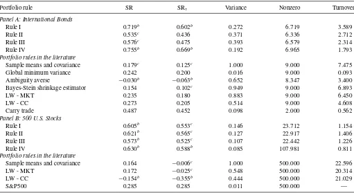
Table 2. Out-of-sample performance of alternative portfolio rules on foreign exchange rates and U.S. stocks
Portfolio rule SR SRτ Variance Nonzero Turnover
Panel A: International Bonds
Rule I 0.719b 0.602b 0.272 6.719 3.589
Rule II 0.535c 0.436 0.371 6.336 2.712
Rule III 0.576c 0.475 0.393 6.579 2.314
Rule IV 0.755b 0.669b 0.192 6.965 1.793
Portfolio rules in the literature
Sample means and covariance 0.179c 0.125c 1.000 9.000 7.475
Global minimum variance 0.242 0.200 0.016 9.000 0.093 Ambiguity averse −0.030b
−0.063b 0.652 8.347 3.400
Bayes-Stein shrinkage estimator 0.154 0.102c 0.949 9.000 6.893
LW - MKT 0.235 0.180 0.883 9.000 6.450
LW - CC 0.273 0.205 0.514 9.000 4.608
Carry trade 0.487 0.452 0.098 2.000 0.562
Panel B: 500 U.S. Stocks
Rule I 0.605b 0.553c 0.146 23.712 1.154
Rule II 0.621b 0.565c 0.127 22.917 1.406
Rule III 0.573b 0.525c 0.107 22.442 1.226
Rule IV 0.630b 0.588b 0.085 107.981 0.811
Portfolio rules in the literature
Sample means and covariance 0.164 −0.006c 1.000 500.000 22.596
LW - MKT 0.172 −0.025c 0.548 500.000 20.314
LW - CC −0.154b
−0.355b 0.444 500.000 21.029
S&P500 0.285 0.285 0.011 500.000 —
NOTE: The superscripts a, b, and c denote statistical significance at the 1%, 5%, and 10% level, respectively.
where the former strategy is designed to minimize portfolio variance, and the latter one purely explores the forward pre-mium anomaly and is free of estimation risk. On average, less than seven assets are included in each of four norm-constrained portfolios. “Rule II” and “Rule III,” however, show limited im-provements over carry trade, which indicates factor model and constant-correlation model are less suitable for modeling co-movements of currencies. “Rule I” and “Rule IV” with data-driven constraints perform best in terms of Sharp ratios, but “Rule IV” has smaller variance and turnover.
In the last empirical example, we consider a large number of individual stocks from the U.S. market. For each month between January 1986 and December 2013, we create a pool of stocks from common stocks listed on the NYSE or NASDAQ. Stocks in this pool have prices greater than five dollars, market capi-talizations more than the 80th percentile of the size distribution of all firms, and monthly return data for all the immediately preceding 10 years. Both stock prices and returns have been adjusted for dividend and stock splits. We then randomly select 500 stocks from this pool of stock, estimate expected returns and covariance matrix based on a 10-year rolling window, and for-mulate portfolios whose returns are realized over the following one-month holding period.5
We use the passively managed S&P 500 index over the same evaluation period as the benchmark. This is a standard bench-mark for the U.S. equity bench-market, which is accessible to both in-stitutional investors and individual investors through Vanguard 500 Index Fund, among other alternatives. WhenN > T, how-ever, the level of ambiguity aversionǫin ambiguity averse port-folio cannot be derived. Moreover, global minimum-variance portfolio and the portfolio based on Bayes-Stein estimator can-not estimate the covariance matrix. Therefore we only evaluate and report the performance of the remaining active portfolio strategies.
From January 1986 to December 2013, the returns of S&P500 over the risk-free rate (proxied by the 3-month Treasury Bill rate) have an average of 4.36% and a standard deviation of 15.32%, leading to a Sharpe ratio of 0.285. As can be seen from the Panel B ofTable 2, all norm-constrained portfolios significantly outperform the market index, even though trading frictions are considered. Given the same amount of risk, the excess returns from norm-constrained portfolios could be more than doubled. On average, more than 20 assets are selected by “Rule I,” “Rule II,” and “Rule III,” and more than 100 assets are selected by “Rule IV,” corresponding to sparsities of around 90% and 80%, respectively. “Rule IV” again has the lowest turnover and variance.
To provide a visual illustration of the results,Figure 2plots the cumulative wealth of strategy “Rule IV” (red line) relative to the benchmark (blue line) for international bond portfolios (Figure 2(a)) or individual stock portfolios (Figure 2(b)). In both figures initial wealth is set at $1, which grows at the monthly return of different portfolio strategies. The figures show emphat-ically the superior performance of the norm-constrained portfo-lio, and provide an interesting view about which time period a particular strategy performs well. This is important because our
5See, for example, Jagannathan and Ma (2003). We thank the Associate Editor
for pointing this out.
sample includes the demise of Long Term Capital Management in 1998, the dot-com bubble of the late 1990s as well as the subprime mortgage crisis between 2007 and 2009. We can see that, both portfolios’ cumulative wealth tumbled during crises, but that of the norm-constrained portfolio increased quickly in other periods. From December 2011 to December 2013, for ex-ample, the return of S&P500 index is about 45%, while it is about 80% for the norm-constrained portfolio.6
6. CONCLUSIONS
The classic portfolio selection is an optimization problem without explicitly addressing parameter uncertainty, and usu-ally delivers abysmal out-of-sample performance. In this arti-cle we develop a regression approach for the portfolio choice problem, and propose to constrain portfolio weights directly to achieve sparsity and stability. Sparse portfolio sets small port-folio weights to zero, which optimizes the budget allocation by focusing on assets that are expected to make substantial con-tributions to diversification. The stability of a portfolio, on the other hand, mitigates the impact of estimation errors when in-verting the estimated covariance matrix, and tends to produce stable and diversified portfolio weights.
In light of the regression analysis, we show that under cer-tain conditions, the doubly-constrained portfolios are related to the classic solution by scaling and shifting the classic portfo-lio rule. When the number of assets is large, this strategy is particularly helpful, since it overcomes extreme and unstable portfolio weights implied by poor sample estimates. We further show how new portfolio rules are connected to other portfo-lio rules in the literature. Empirical analyses confirm that the proposed portfolio strategies have better out-of-sample perfor-mance with relatively low turnovers. These results are robust against transaction costs.
In practice, the size of estimation window for portfolio choice problems is limited for two reasons. First, the data are not al-ways available for a longer period especially if the data fre-quency is low. Second, in general moments of excess returns are time-varying. Defining a reasonable length of estimation window is a way of approximating and estimating time-varying return characteristics. As a result, increasing the length of esti-mation window may increase the chance of model misspecifica-tion. Therefore, with limited observations for estimations, norm-constrained portfolios serve as promising investment strategies when the number of assets is large.
APPENDIX: PROOFS
Proof of Proposition 1. Linear model theory estimates regression coefficientswby
ˆ
wOLS =argmin
w {
(y−Xw)T(y −Xw)}
=argmax
w
wT(XTy)−1 2w
T XTXw
.
6The same period, however, was a tough one for the currency market. As central banks in developed countries fight the financial crisis and keep low interest rates, carry trade opportunities are wiped out. This period ends up with the collapse of FX Concepts, once the world’s biggest currency hedge fund.
By matching the coefficients in (1),Xandycan be defined, so that
the least squares problem (2) coincides with the portfolio selection
problem (1).
Proof of Proposition 2. Note that
ˆ
g , this is equivalent to a ridge regression
or Tikhonov regularization problem (Tikhonov and Arsenin1979): ˆw=
argmin
implies that there exist a lower-triangular matrixLand a diagonal matrix
C such that 2λˆg=LCLT. Therefore according to the Woodbury
Proof of Proposition 3. The solution follows from the equivalent problem of (20):
Due to the Minkowski inequality, N
j=1 |wˆµ,j| = ||wˆµ ||1 =
The author is very grateful to the Editor, the Associate Edi-tor, and three anonymous referees for providing insightful and detailed suggestions that significantly improved the article. The author also thanks Thomas Cosimano, Ilias Tsiakas, and Guofu Zhou for constructive discussions.
[Received June 2013. Revised July 2014.]
REFERENCES
Andersen, T. G., Bollerslev, T., Diebold, F. X., and Ebens, H. (2001), “The Distribution of Realized Stock Return Volatility,”Journal of Financial Eco-nomics, 61, 43–76. [385]
Bai, J., and Ng, S. (2008), “Forecasting Economic Time Series Using Targeted Predictors,”Journal of Econometrics, 146, 304–317. [383]
Behr, P., Guettler, A., and Miebs, F. (2013), “On Portfolio Optimization: Im-posing the Right Constraints,”Journal of Banking and Finance, 1232–1242. [381]
Berger, J. O. (1985),Statistical Decision Theory and Bayesian Analysis, New York: Springer. [386]
Bertsimas, D., and Lo, A. W. (1998), “Optimal Control of Execution Costs,” Journal of Financial Markets, 1, 1–50. [387]
Brandt, M. W. (2009), “Portfolio Choice Problems,” inHandbook of Financial Econometrics(Vol. 1), Amsterdam, the Netherlands: Elsevier, pp. 269–336. [381,382,383]
Britten-Jones, M. (1999), “The Sampling Error in Estimates of Mean-Variance Efficient Portfolio Weights,”The Journal of Finance, 54, 655– 671. [381,382,383]
Brodie, J., Daubechies, I., De Mol, C., Giannone, D., and Loris, I. (2009), “Sparse and Stable Markowitz Portfolios,” Proceedings of the National Academy of Sciences, 106, 12267–12272. [381,383]
De Mol, C., Giannone, D., and Reichlin, L. (2008), “Forecasting Using a Large Number of Predictors: Is Bayesian Shrinkage a Valid Alternative to Principal Components?,”Journal of Econometrics, 146, 318–328. [383]
Della Corte, P., Sarno, L., and Tsiakas, I. (2009), “An Economic Evaluation of Empirical Exchange Rate Models,”Review of Financial Studies, 22, 3491– 3530. [387,388]
——— (2011), “Spot and Forward Volatility in Foreign Exchange,”Journal of Financial Economics, 100, 496–513. [388]
DeMiguel, V., Garlappi, L., Nogales, F. J., and Uppal, R. (2009), “A Generalized Approach to Portfolio Optimization: Improving Perfor-mance by Constraining Portfolio Norms,”Management Science, 55, 798– 812. [381,385,387]
DeMiguel, V., Garlappi, L., and Uppal, R. (2009), “Optimal Versus Naive Di-versification: How Inefficient is the 1/N Portfolio Strategy?,”Review of Financial Studies, 22, 1915–1953. [387,388]
Efron, B., Hastie, T., Johnstone, I., and Tibshirani, R. (2004), “Least Angle Regression,”The Annals of Statistics, 32, 407–499. [385]
Fan, J., Liao, Y., and Mincheva, M. (2013), “Large Covariance Estimation by Thresholding Principal Orthogonal Complements,”Journal of the Royal Statistical Society,Series B, 75, 603–680. [386]
Fan, J., Zhang, J., and Yu, K. (2012), “Vast Portfolio Selection With Gross-exposure Constraints,”Journal of the American Statistical Association, 107, 592–606. [381,383]
Frost, P. A., and Savarino, J. E. (1986), “An Empirical Bayes Approach to Effi-cient Portfolio Selection,”Journal of Financial and Quantitative Analysis, 21, 293–305. [381]
Garlappi, L., Uppal, R., and Wang, T. (2007), “Portfolio Selection With Param-eter and Model Uncertainty: A Multi-Prior Approach,”Review of Financial Studies, 20, 41–81. [381,382,383,386,387]
Jagannathan, R., and Ma, T. (2003), “Risk Reduction in Large Portfolios: Why Imposing the Wrong Constraints Helps,”The Journal of Finance, 58, 1651– 1684. [381,390]
Jones, C. (2002), “A Century of Stock Market Liquidity and Trading Costs,” unpublished working paper, Columbia University. [388]
Jorion, P. (1986), “Bayes-Stein Estimation for Portfolio Analysis,”Journal of Financial and Quantitative Analysis, 21, 279–292. [381,382,386,387] ——— (1991), “The Pricing of Exchange Rate Risk in the Stock Market,”
Journal of Financial and Quantitative Analysis, 26, 363–376. [386]
Kan, R., and Zhou, G. (2007), “Optimal Portfolio Choice With Param-eter Uncertainty,” Journal of Financial and Quantitative Analysis, 42, 621. [382,383,386]
Klein, R. W., and Bawa, V. S. (1976), “The Effect of Estimation Risk on Optimal Portfolio Choice,”Journal of Financial Economics, 3, 215–231. [386]
Kourtis, A., Dotsis, G., and Markellos, R. N. (2012), “Parameter Uncertainty in Portfolio Selection: Shrinking the Inverse Covariance Matrix,”Journal of Banking and Finance, 36, 2522–2531. [387]
Ledoit, O., and Wolf, M. (2003), “Improved Estimation of the Covariance Matrix of Stock Returns With an Application to Portfolio Selection,”Journal of Empirical Finance, 10, 603–621. [381,382,383,384,385,387]
——— (2004), “Honey, I Shrunk the Sample Covariance Matrix,”Journal of Portfolio Management, 30, 110–119. [381,382,384,385,387]
——– (2008), “Robust Performance Hypothesis Testing With the Sharpe Ratio,” Journal of Empirical Finance, 15, 850–859. [387]
Li, J., Tsiakas, I., and Wang, W. (2014), “Predicting Exchange Rates Out of Sample: Can Economic Fundamentals Beat the Random Walk?,”Journal of Financial Econometrics, nbu007. [387]
Menkhoff, L., Sarno, L., Schmeling, M., and Schrimpf, A. (2012), “Carry Trades and Global Foreign Exchange Volatility,”The Journal of Finance, 67, 681– 718. [388]
Neely, C. J., Weller, P. A., and Ulrich, J. M. (2009), “The Adaptive Markets Hypothesis: Evidence From the Foreign Exchange Market,”Journal of Fi-nancial and Quantitative Analysis, 44, 467–488. [388]
Stambaugh, R. F. (1997), “Analyzing Investments Whose Histories Differ in Length,”Journal of Financial Economics, 45, 285–331. [386]
Stein, C. (1956), “Inadmissibility of the Usual Estimator for the Mean of a Multi-variate Normal Distribution,”Proceedings of the Third Berkeley Symposium on Mathematical Statistics and Probability, 1, 197–206. [386]
Tibshirani, R. (1996), “Regression Shrinkage and Selection via the Lasso,” Journal of the Royal Statistical Society,Series B, 267–288. [383] Tikhonov, A. N., and Arsenin, V. Y. (1979),Methods for Solving Ill-Posed
Problems,Scripta Series in Mathematics, New York: Scripta Mathematics. [391]
Zou, H., and Hastie, T. (2005), “Regularization and Variable Selection via the Elastic Net,”Journal of the Royal Statistical Society,Series B, 67, 301–320. [385]