LAMPIRAN A
HASIL UJI MUTU FISIK GRANUL
Mutu fisik yang diuji
Batch
Formula Tablet Propranolol HCl
LAMPIRAN B
HASIL UJI KEKERASAN TABLET SUBLINGUAL
PROPRANOLOL HCl
Batch I
No Kekerasan Tablet Propranolol (kp)
Batch II
No Kekerasan Tablet Propranolol (kp)
Formula A Formula B Formula C Formula D
1 6,3 4,9 6,9 5,1
2 6,4 4,6 6,7 5,5
3 6,1 4,5 6,9 5,4
4 6,4 4,6 6,8 5,1
5 6,1 4,6 6,8 5,3
6 5,9 4,9 6,9 5,0
7 6,2 4,8 6,5 5,5
8 6,1 4,7 6,6 5,4
9 6,2 4,8 6,8 5,2
10 6,2 4,7 6,7 5,4
X
SD 6,19 ± 0,15 4,71 ± 0,14 6,76 ± 0,13 5,29 ± 0,18 SD rel73 Batch III
No Kekerasan Tablet Propranolol (kp)
Formula A Formula B Formula C Formula D
1 6,2 4,6 6,8 5,2
2 6,2 4,6 6,8 5,4
3 5,9 4,8 6,7 5,6
4 6,2 4,7 6,7 5,5
5 5,8 4,8 6,8 5,7
6 6,1 4,5 6,8 5,6
7 5,8 4,5 6,6 5,2
8 6,2 4,9 6,9 5,3
9 6,1 4,7 6,9 5,2
10 5,7 4,8 6,7 5,3
X
SD 6,02 ± 0,20 4,69 ± 0,14 6,77 ± 0,09 5,40 ± 0,19 SD relLAMPIRAN C
HASIL UJI KERAPUHAN TABLET SUBLINGUAL
LAMPIRAN D
HASIL UJI WAKTU HANCUR TABLET SUBLINGUAL
PROPRANOLOL HCl
Replikasi Waktu Hancur (menit)
Formula A Formula B Formula C Formula D
1 24 3 28 11
2 28 3 26 6
3 28 4 28 11
LAMPIRAN E
HASIL UJI KESERAGAMAN KANDUNGAN TABLET PROPRANOLOL HCl
Hasil Uji Keragaman Kandungan Tablet Formula A Batch I
Hasil Uji Keragaman Kandungan Tablet Formula A Batch II
Hasil Uji Keragaman Kandungan Tablet Formula A Batch III
Hasil Uji Keragaman Kandungan Tablet Formula B Batch I
Hasil Uji Keragaman Kandungan Tablet Formula B Batch II
Hasil Uji Keragaman Kandungan Tablet Formula B Batch III
Hasil Uji Keragaman Kandungan Tablet Formula C Batch I
80 Hasil Uji Keragaman Kandungan Tablet Formula C Batch II
Abs C sampel W sampel C teoritis Kadar (%)
Hasil Uji Keragaman Kandungan Tablet Formula C Batch III
Hasil Uji Keragaman Kandungan Tablet Formula D Batch I
Hasil Uji Keragaman Kandungan Tablet Formula D Batch II
Hasil Uji Keragaman Kandungan Tablet Formula D Batch III
Abs C sampel W sampel C teoritis Kadar (%)
0,369 14,96 302,5 16,27 91,95
0,371 15,07 300,4 16,04 93,95
0,362 14,59 300,9 16,10 90,62
0,387 15,91 303,7 16,40 97,01
0,374 15,22 302,8 16,30 93,37
0,368 14,91 300,6 16,06 92,84
0,385 15,81 303,5 16,38 96,52
0,376 15,33 302,1 16,22 94,51
0,372 15,12 303,7 16,36 92,42
0,379 15,49 300,4 16,04 96,57
X 93,98
SD 2,16
LAMPIRAN F
85 LAMPIRAN G
HASIL UJI DISOLUSI TABLET SUBLINGUAL PROPRANOLOL
HCl PADA T = 15 MENIT
LAMPIRAN H
CONTOH PERHITUNGAN
Contoh perhitungan sudut diam:
Formula (-1):
Contoh perhitungan indeks kompresibilitas:
Formula (-1) :
Berat gelas = 119,14 g (W1)
Berat gelas + granul = 168,16 g (W2) V1 = 100 ml
Bj nyata =
Contoh perhitungan akurasi & presisi:
Perolehan
Replikasi Konsentrasi Absorbansi Konsentrasi Teoritis Kembali KV
(µg/ml) (µg/ml) (%) (%) Konsentrasi sebenarnya = 12,74 ppm
88 Konsentrasi teoritis = 12,82 ppm
% perolehan kembali = (konsentrasi sebenarnya / konsentrasi teoritis) x 100%
Contoh perhitungan % obat terlepas:
% obat terlepas = x 100%
LAMPIRAN I
SERTIFIKAT ANALISIS BAHAN
SERTIFIKAT ANALISIS BAHAN
LAMPIRAN J
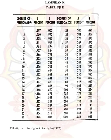
94 LAMPIRAN K
TABEL UJI R
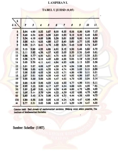
LAMPIRAN L
LAMPIRAN M
97 LAMPIRAN N
HASIL UJI STATISTIK KEKERASAN TABLET ANTAR FORMULA
Descriptives Kekerasan
N Mean Std. Deviation Std. Error
95% Confidence Interval for Mean
Minimum Maximum Lower Bound Upper Bound
Formula A 3 6,1300 ,09539 ,05508 5,8930 6,3670 6,02 6,19
Formula B 3 4,7200 ,03606 ,02082 4,6304 4,8096 4,69 4,76
Formula C 3 6,7900 ,04359 ,02517 6,6817 6,8983 6,76 6,84
Formula D 3 5,4567 ,20108 ,11609 4,9572 5,9562 5,29 5,68
Total 12 5,7742 ,81001 ,23383 5,2595 6,2888 4,69 6,84
Test of Homogeneity of Variances
Kekerasan
Levene Statistic df1 df2 Sig.
4.357 3 8 .043
ANOVA Kekerasan
Sum of Squares df Mean Square F Sig.
Between Groups 7.112 3 2.371 179.819 .000
Within Groups .105 8 .013
Total 7.217 11
Multiple Comparisons Lower Bound Upper Bound
Formula D Formula A -,67333* ,09375 .000 -,8895 -,4571
Formula B ,73667* ,09375 .000 ,5205 ,9529
Formula C -1,33333* ,09375 .000 -1,5495 -1,1171
*. The mean difference is significant at the 0.05 level.
LAMPIRAN O
HASIL UJI STATISTIK KERAPUHAN TABLET ANTAR FORMULA
Descriptives Kerapuhan
N Mean Std. Deviation Std. Error
95% Confidence Interval for Mean
Minimum Maximum Lower Bound Upper Bound
Formula A 3 ,6067 ,09238 ,05333 ,3772 ,8361 ,50 ,66
Formula B 3 ,6167 ,09238 ,05333 ,3872 ,8461 ,51 ,67
Formula C 3 ,1667 ,00577 ,00333 ,1523 ,1810 ,16 ,17
Formula D 3 ,4967 ,00577 ,00333 ,4823 ,5110 ,49 ,50
Total 12 ,4717 ,19840 ,05727 ,3456 ,5977 ,16 ,67
Test of Homogeneity of Variances
Kerapuhan
Levene Statistic df1 df2 Sig.
9.339 3 8 .005
ANOVA Kerapuhan
Sum of Squares df Mean Square F Sig.
Between Groups .399 3 .133 31.027 .000
Within Groups .034 8 .004
Total .433 11
10
Multiple Comparisons Lower Bound Upper Bound
Formula D Formula A -,11000 ,05344 .074 -,2332 ,0132
Formula B -,12000 ,05344 .055 -,2432 ,0032
Formula C ,33000* ,05344 .000 ,2068 ,4532
*. The mean difference is significant at the 0.05 level.
LAMPIRAN P
HASIL UJI STATISTIK WAKTU HANCUR TABLET ANTAR FORMULA
Descriptives Waktuhancur
N Mean Std. Deviation Std. Error
95% Confidence Interval for Mean
Minimum Maximum Lower Bound Upper Bound
Formula A 3 26,6667 2,30940 1,33333 20,9298 32,4035 24,00 28,00
Formula B 3 3,3333 ,57735 ,33333 1,8991 4,7676 3,00 4,00
Formula C 3 27,3333 1,15470 ,66667 24,4649 30,2018 26,00 28,00
Formula D 3 9,3333 2,88675 1,66667 2,1622 16,5044 6,00 11,00
Total 12 16,6667 11,14641 3,21769 9,5846 23,7488 3,00 28,00
Test of Homogeneity of Variances Waktuhancur
Levene Statistic df1 df2 Sig.
4.638 3 8 .037
ANOVA Waktuhancur
Sum of Squares df Mean Square F Sig.
Between Groups 1336.000 3 445.333 116.174 .000
Within Groups 30.667 8 3.833
Total 1366.667 11
Multiple Comparisons Lower Bound Upper Bound
Formula D Formula A -17,33333* 1,59861 .000 -21,0197 -13,6469
Formula B 6,00000* 1,59861 .006 2,3136 9,6864
Formula C -18,00000* 1,59861 .000 -21,6864 -14,3136
*. The mean difference is significant at the 0.05 level.
LAMPIRAN Q
HASIL UJI STATISTIK PERSEN DISOLUSI TABLET ANTAR FORMULA
Descriptives Disolusi
N Mean Std. Deviation Std. Error
95% Confidence Interval for Mean
Minimum Maximum Lower Bound Upper Bound
Formula A 3 10,5233 ,30139 ,17401 9,7746 11,2720 10,24 10,84
Formula B 3 93,4367 ,15631 ,09025 93,0484 93,8250 93,27 93,58
Formula C 3 7,9667 ,13317 ,07688 7,6359 8,2975 7,82 8,08
Formula D 3 82,5933 ,15631 ,09025 82,2050 82,9816 82,45 82,76
Total 12 48,6300 41,34184 11,93436 22,3626 74,8974 7,82 93,58
Test of Homogeneity of Variances Disolusi
Levene Statistic df1 df2 Sig.
.847 3 8 .506
ANOVA Disolusi
Sum of Squares df Mean Square F Sig.
Between Groups 18800.310 3 6266.770 159223.462 .000
Within Groups .315 8 .039
Total 18800.625 11
Multiple Comparisons Lower Bound Upper Bound
Formula D Formula A 72,07000* ,16198 .000 71,6965 72,4435
Formula B -10,84333* ,16198 .000 -11,2169 -10,4698
Formula C 74,62667* ,16198 .000 74,2531 75,0002
*. The mean difference is significant at the 0.05 level.
11
LAMPIRAN R
HASIL ANOVA UJI KEKERASAN PADA PROGRAM DESIGN EXPERT
Response 1 Kekerasan
ANOVA for selected factorial model
Analysis of variance table [Partial sum of squares - Type III]
Sum of Mean F p-value
The Model F-value of 179.82 implies the model is significant. There is only a 0.01% chance that a "Model F-Value" this large could occur due to noise. Values of "Prob > F" less than 0.0500 indicate model terms are significant. In this case A, B are significant model terms.
Values greater than 0.1000 indicate the model terms are not significant.
If there are many insignificant model terms (not counting those required to support hierarchy),
1
1
model reduction may improve your model.
Std. Dev. 0.11 R-Squared 0.9854
Mean 5.77 Adj R-Squared 0.9799
C.V. % 1.99 Pred R-Squared 0.9671
PRESS 0.24 Adeq Precision 31.226
The "Pred R-Squared" of 0.9671 is in reasonable agreement with the "Adj R-Squared" of 0.9799. "Adeq Precision" measures the signal to noise ratio. A ratio greater than 4 is desirable. Your ratio of 31.226 indicates an adequate signal. This model can be used to navigate the design space.
Coefficient Standard 95% CI 95% CI
Final Equation in Terms of Coded Factors:
Kekerasan =
+5.77
-0.69 * A
11
+0.35 * B
+0.019 * A * B
Final Equation in Terms of Actual Factors:
Kekerasan =
+6.32229
-0.35729 * Xanthan gum
+0.16021 * PVP K-30
+4.79167E-003 * Xanthan gum * PVP K-30
The Diagnostics Case Statistics Report has been moved to the Diagnostics Node. In the Diagnostics Node, Select Case Statistics from the View Menu.
Proceed to Diagnostic Plots (the next icon in progression). Be sure to look at the:
1) Normal probability plot of the studentized residuals to check for normality of residuals. 2) Studentized residuals versus predicted values to check for constant error.
3) Externally Studentized Residuals to look for outliers, i.e., influential values. 4) Box-Cox plot for power transformations.
If all the model statistics and diagnostic plots are OK, finish up with the Model Graphs icon.
11
LAMPIRAN S
HASIL ANOVA UJI KERAPUHAN PADA DESIGN EXPERT
Response 2 Kerapuhan
ANOVA for selected factorial model
Analysis of variance table [Partial sum of squares - Type III]
Sum of Mean F p-value
The Model F-value of 31.03 implies the model is significant. There is only a 0.01% chance that a "Model F-Value" this large could occur due to noise. Values of "Prob > F" less than 0.0500 indicate model terms are significant. In this case A, B, AB are significant model terms.
Values greater than 0.1000 indicate the model terms are not significant.
If there are many insignificant model terms (not counting those required to support hierarchy),
11
model reduction may improve your model.
Std. Dev. 0.065 R-Squared 0.9209
Mean 0.47 Adj R-Squared 0.8912
C.V. % 13.88 Pred R-Squared 0.8219
PRESS 0.077 Adeq Precision 11.909
The "Pred R-Squared" of 0.8219 is in reasonable agreement with the "Adj R-Squared" of 0.8912. "Adeq Precision" measures the signal to noise ratio. A ratio greater than 4 is desirable. Your ratio of 11.909 indicates an adequate signal. This model can be used to navigate the design space.
Coefficient Standard 95% CI 95% CI
Final Equation in Terms of Coded Factors:
Kerapuhan =
+0.47
+0.085 * A
11
-0.14 * B
+0.080 * A * B
Final Equation in Terms of Actual Factors:
Kerapuhan =
+0.73417
-0.017500 * Xanthan gum
-0.13000 * PVP K-30
+0.020000 * Xanthan gum * PVP K-30
The Diagnostics Case Statistics Report has been moved to the Diagnostics Node. In the Diagnostics Node, Select Case Statistics from the View Menu.
Proceed to Diagnostic Plots (the next icon in progression). Be sure to look at the:
1) Normal probability plot of the studentized residuals to check for normality of residuals. 2) Studentized residuals versus predicted values to check for constant error.
3) Externally Studentized Residuals to look for outliers, i.e., influential values. 4) Box-Cox plot for power transformations.
If all the model statistics and diagnostic plots are OK, finish up with the Model Graphs icon.
11
LAMPIRAN T
HASIL ANOVA UJI WAKTU HANCUR PADA DESIGN EXPERT
Use your mouse to right click on individual cells for definitions.
Response 3 Waktu hancur
ANOVA for selected factorial model
Analysis of variance table [Partial sum of squares - Type III]
Sum of Mean F p-value
The Model F-value of 116.17 implies the model is significant. There is only a 0.01% chance that a "Model F-Value" this large could occur due to noise. Values of "Prob > F" less than 0.0500 indicate model terms are significant. In this case A, B, AB are significant model terms.
Values greater than 0.1000 indicate the model terms are not significant.
If there are many insignificant model terms (not counting those required to support hierarchy),
1
model reduction may improve your model.
Std. Dev. 1.96 R-Squared 0.9776
Mean 16.67 Adj R-Squared 0.9691
C.V. % 11.75 Pred R-Squared 0.9495
PRESS 69.00 Adeq Precision 21.232
The "Pred R-Squared" of 0.9495 is in reasonable agreement with the "Adj R-Squared" of 0.9691. "Adeq Precision" measures the signal to noise ratio. A ratio greater than 4 is desirable. Your ratio of 21.232 indicates an adequate signal. This model can be used to navigate the design space.
Coefficient Standard 95% CI 95% CI
Final Equation in Terms of Coded Factors:
Waktu hancur =
+16.67
-10.33 * A
+1.67 * B
+1.33 * A * B
Final Equation in Terms of Actual Factors:
Waktu hancur =
+32.66667
-6.16667 * Xanthan gum
-0.16667 * PVP K-30
+0.33333 * Xanthan gum * PVP K-30
The Diagnostics Case Statistics Report has been moved to the Diagnostics Node. In the Diagnostics Node, Select Case Statistics from the View Menu.
Proceed to Diagnostic Plots (the next icon in progression). Be sure to look at the:
1) Normal probability plot of the studentized residuals to check for normality of residuals. 2) Studentized residuals versus predicted values to check for constant error.
3) Externally Studentized Residuals to look for outliers, i.e., influential values. 4) Box-Cox plot for power transformations.
If all the model statistics and diagnostic plots are OK, finish up with the Model Graphs icon.
LAMPIRAN U
HASIL ANOVA UJI PERSEN DISOLUSI PADA DESIGN EXPERT
Use your mouse to right click on individual cells for definitions.
Response 4 Persen Disolusi
ANOVA for selected factorial model
Analysis of variance table [Partial sum of squares - Type III]
Sum of Mean F p-value
Source Squares df Square Value Prob > F
Model 18800.31 3 6266.77 1.592E+005 < 0.0001 significant A-Xanthan gum 18614.14 1 18614.14 4.729E+005 < 0.0001
B-PVP K-30 134.67 1 134.67 3421.64 < 0.0001 AB 51.50 1 51.50 1308.53 < 0.0001
Pure Error 0.31 8 0.039
Cor Total 18800.63 11
The Model F-value of 159223.46 implies the model is significant. There is only a 0.01% chance that a "Model F-Value" this large could occur due to noise. Values of "Prob > F" less than 0.0500 indicate model terms are significant. In this case A, B, AB are significant model terms.
Values greater than 0.1000 indicate the model terms are not significant.
If there are many insignificant model terms (not counting those required to support hierarchy),
model reduction may improve your model.
Std. Dev. 0.20 R-Squared 1.0000
Mean 48.63 Adj R-Squared 1.0000
C.V. % 0.41 Pred R-Squared 1.0000
PRESS 0.71 Adeq Precision 746.201
The "Pred R-Squared" of 1.0000 is in reasonable agreement with the "Adj R-Squared" of 1.0000. "Adeq Precision" measures the signal to noise ratio. A ratio greater than 4 is desirable. Your ratio of 746.201 indicates an adequate signal. This model can be used to navigate the design space.
Coefficient Standard 95% CI 95% CI
Final Equation in Terms of Coded Factors:
Persen Disolusi =
+48.63
+39.38 * A
-3.35 * B
-2.07 * A * B
Final Equation in Terms of Actual Factors:
Persen Disolusi =
-10.08375
+21.24625 * Xanthan gum -0.12125 * PVP K-30
-0.51792 * Xanthan gum * PVP K-30
The Diagnostics Case Statistics Report has been moved to the Diagnostics Node. In the Diagnostics Node, Select Case Statistics from the View Menu.
Proceed to Diagnostic Plots (the next icon in progression). Be sure to look at the:
1) Normal probability plot of the studentized residuals to check for normality of residuals. 2) Studentized residuals versus predicted values to check for constant error.
3) Externally Studentized Residuals to look for outliers, i.e., influential values. 4) Box-Cox plot for power transformations.
If all the model statistics and diagnostic plots are OK, finish up with the Model Graphs icon.
LAMPIRAN V
UJI F KURVA BAKU
Uji Kesamaan Regresi (Aquadest)
REPLIKASI 1
8,016 0,259 64,256256 0,067081 2,076144
14,028 0,374 196,784784 0,139876 5,246472
20,040 0,486 401,6016 0,236196 9,73944
26,052 0,599 678,706704 0,358801 15,605148
32,064 0,710 1028,100096 0,5041 22,76544
38,076 0,823 1449,781776 0,677329 31,336548 3823,247232 2,005883 87,069792
REPLIKASI 2
8,016 0,239 64,256256 0,057121 1,915824
14,028 0,363 196,784784 0,131769 5,092164
20,040 0,459 401,6016 0,210681 9,19836
ii
8,032 0,239 64,513024 0,057121 1,919648
14,056 0,360 197,571136 0,1296 5,06016
20,08 0,465 403,2064 0,216225 9,3372
26,104 0,585 681,418816 0,342225 15,27084 32,128 0,715 1032,208384 0,511225 22,97152 38,152 0,825 1455,575104 0,680625 31,4754
3838,524928 1,954445 86,299824
X2 XY Y2 N SSi RDF
Regresi I 3823,247232 87,069792 2,005883 7 0,0229747 6 Regresi II 3823,247232 84,404472 1,877306 7 0,0139384 6 Regresi III 3838,524928 86,299824 1,954445 7 0,014205 6
11485,01939 257,774088 5,837634 0,0511181
Ssc = 0,0520556 F hitung = 0,0825
LAMPIRAN W
UJI F KURVA BAKU
Uji Kesamaan Regresi (Dapar Fosfat pH 6,8)
REPLIKASI 1
65,26 1,686 4258,8676 2,842596 110,02836
80,32 2,073 6451,3024 4,297329 166,50336
95,38 2,177 9097,3444 4,739329 207,64226
23990,7808 15,695967 608,68504
REPLIKASI 2
35,07 1,226 1229,9049 1,503076 42,99582
50,10 1,494 2510,01 2,232036 74,8494
65,13 1,740 4241,9169 3,0276 113,3262
80,16 2,074 6425,6256 4,301476 166,25184
95,19 2,347 9061,1361 5,508409 223,41093
REPLIKASI 3
35,07 1,111 1229,9049 1,234321 38,96277
50,10 1,384 2510,01 1,915456 69,3384
65,13 1,672 4241,9169 2,795584 108,89736
80,16 1,997 6425,6256 3,988009 160,07952
95,19 2,303 9061,1361 5,303809 219,22257
350,7 9,604 23895,2952 16,065368 615,27309
X2 XY Y2 N SSi RDF Regresi I 23990,7808 608,68504 15,695967 7 0,25263979 6 Regresi II 23895,2952 640,23291 17,455126 7 0,301197764 6 Regresi III 23895,2952 615,27309 16,065368 7 0,222877999 6
71781,3712 1864,19104 49,216461 0,776715553
Ssc = 0,802670966 F hitung = 0,1504