Combinatorics 2nd ed. R. Merris Free ebook download for u

(1)

(2)

(3)

WILEY-INTERSCIENCE

SERIES IN DISCRETE MATHEMATICS AND OPTIMIZATION ADVISORY EDITORS

RONALD L. GRAHM

University of California at San Diego, U.S.A.

JAN KAREL LENSTRA

Department of Mathematics and Computer Science,

Eindhoven University of Technology, Eindhoven, The Netherlands

JOEL H. SPENCER

Courant Institute, New York, New York, U.S.A.

(4)

Combinatorics

SECOND EDITION

RUSSELL MERRIS

California State University, Hayward

(5)

No part of this publication may be reproduced, stored in a retrieval system or transmitted in any form or by any means, electronic, mechanical, photocopying, recording, scanning or otherwise, except as permitted under Sections 107 or 108 of the 1976 United States Copyright Act, without either the prior written permission of the Publisher, or authorization through payment of the appropriate per-copy fee to the Copyright Clearance Center, 222 Rosewood Drive, Danvers, MA 01923, (978) 750-8400, fax (978) 750-4744. Requests to the Publisher for permission should be addressed to the Permissions Department, John Wiley & Sons, Inc., 605 Third Avenue, New York, NY 10158-0012,

(212) 850-6011, fax: (212) 850-6008, E-Mail: PERMREQ@WILEY.COM.

For ordering and customer service, call 1-800-CALL-WILEY.

Library of Congress Cataloging-in-Publication Data:

Merris, Russell, 1943–

Combinatorics / Russell Merris.–2nd ed.

p. cm. – (Wiley series in discrete mathematics and optimization) Includes bibliographical references and index.

ISBN-0-471-26296-X (acid-free paper) 1. Combinatorial analysis I. Title. II. Series.

QA164.M47 2003

5110_.6–dc21 _2002192250

Printed in the United States of America.

(6)

(7)

(8)

Preface

This book is intended to be used as the text for a course in combinatorics at the level of beginning upper division students. It has been shaped by two goals: to make some fairly deep mathematics accessible to students with a wide range of abilities, interests, and motivations and to create a pedagogical tool useful to the broad spec-trum of instructors who bring a variety of perspectives and expectations to such a course.

The author’s approach to the second goal has been to maximize flexibility. Following a basic foundation in Chapters 1 and 2, each instructor is free to pick and choose the most appropriate topics from the remaining four chapters. As sum-marized in the chart below, Chapters 3 – 6 arecompletely independent of each other. Flexibility is further enhanced by optional sections and appendices, by weaving some topics into the exercise sets of multiple sections, and by identifying various points of departure from each of the final four chapters. (The price of this flexibility is some redundancy, e.g., several definitions can be found in more than one place.)

Chapter 5 Chapter 3 Chapter 4 Chapter 6 Chapter 2

Chapter 1

Turning to the first goal, students using this book are expected to have been exposed to, even if they cannot recall them, such notions as equivalence relations, partial fractions, the Maclaurin series expansion forex_{, elementary row operations,} determinants, and matrix inverses. A course designed around this book should have as specific prerequisites those portions of calculus and linear algebra commonly found among the lower division requirements for majors in the mathematical and computer sciences. Beyond these general prerequisites, the last two sections of Chapter 5 presume the reader to be familiar with thedefinitionsof classical adjoint

(11)

(adjugate) and characteristic roots (eigenvalues) of real matrices, and the first two sections of Chapter 6 make use of reduced row-echelon form, bases, dimension, rank, nullity, and orthogonality. (All of these topics are reviewed in Appendix A3.) Strategies that promote student engagement are a lively writing style, timely and appropriate examples, interesting historical anecdotes, a variety of exercises (tem-pered and enlivened by suitable hints and answers), and judicious use of footnotes and appendices to touch on topics better suited to more advanced students. These are things about which there is general agreement, at least in principle.

There is less agreement about how to focus student energies on attainable objec-tives, in part because focusing on some things inevitably means neglecting others. If the course is approached as alast chanceto expose students to this marvelous sub-ject, it probably will be. If approached more invitingly, as afirstcourse in combi-natorics, it may be. To give some specific examples, highlighted in this book are binomial coefficients, Stirling numbers, Bell numbers, and partition numbers. These topics appear and reappear throughout the text. Beyond reinforcement in the service of retention, the tactic of overarching themes helps foster an image of combinato-rics as a unified mathematical discipline. While other celebrated examples, e.g., Bernoulli numbers, Catalan numbers, and Fibonacci numbers, are generously repre-sented, they appear almost entirely in the exercises. For the sake of argument, let us stipulate that these roles could just as well have been reversed. The issue is that beginning upper division students cannot be expected to absorb, much less

appreci-ate, all of these special arrays and sequences in a single semester. On the other

hand, the flexibility is there for willing admirers to rescue one or more of these justly famous combinatorial sequences from the relative obscurity of the exercises. While the overall framework of the first edition has been retained, everything else has been revised, corrected, smoothed, or polished. The focus of many sections has been clarified, e.g., by eliminating peripheral topics or moving them to the exer-cises. Material new to the second edition includes an optional section on algo-rithms, several new examples, and many new exercises, some designed to guide students to discover and prove nontrivial results for themselves. Finally, the section of hints and answers has been expanded by an order of magnitude.

The material in Chapter 3, Po´lya’s theory of enumeration, is typically found clo-ser to the end of comparable books, perhaps reflecting the notion that it is thelast

thing that should be taught in a junior-level course. The author has aspired, not only to make this theory accessible to students taking a first upper division mathematics course, but to make it possible for the subject to be addressed right after Chapter 2. Its placement in the middle of the book is intended to signal that itcanbe fitted in there, not that it must be. If it seems desirable to cover some but not all of Chapter 3, there are many natural places to exit in favor of something else, e.g., after the appli-cation of Bell numbers to transitivity in Section 3.3, after enumerating the overall number of color patterns in Section 3.5, afterstatingPo´lya’s theorem in Section 3.6, or after proving the theorem at the end of Section 3.6.

(12)

intending to go on to Sections 6.1, 6.2, or 6.4. The material in Section 6.3, touching on mutually orthogonal Latin squares and their connection to finite projective planes, can be covered independently of Sections 1.4, 6.1, and 6.2.

The book contains much more material then can be covered in a single semester. Among the possible syllabi for a one semester course are the following:

Chapters 1, 2, and 4 and Sections 3.1–3.3

Chapters 1 (omitting Sections 1.3, 1.4, & 1.10), 2, and 3, and Sections 5.1 & 5.2

Chapters 1 (omitting Sections 1.3 & 1.10), 2, and 6 and Sections 4.1 – 4.4

Chapters 1 (omitting Sections 1.4 & 1.10) and 2 and Sections 3.1 – 3.3,

4.1 – 4.3, & 6.3

Chapters 1 (omitting Sections 1.3 & 1.4) and 2 and Sections 4.1 – 4.3, 5.1, & 5.3–5.7

Chapters 1 (omitting Sections 1.3, 1.4, & 1.10) and 2 and Sections 4.1 – 4.3, 5.1, 5.3–5.5, & 6.3

Many people have contributed observations, suggestions, corrections, and con-structive criticisms at various stages of this project. Among those deserving special mention are former students David Abad, Darryl Allen, Steve Baldzikowski, Dale Baxley, Stanley Cheuk, Marla Dresch, Dane Franchi, Philip Horowitz, Rhian Merris, Todd Mullanix, Cedide Olcay, Glenn Orr, Hitesh Patel, Margaret Slack, Rob Smedfjeld, and Masahiro Yamaguchi; sometime collaborators Bob Grone, Tom Roby, and Bill Watkins; correspondents Mark Hunacek and Gerhard Ringel; reviewers Rob Beezer, John Emert, Myron Hood, Herbert Kasube, Andre´ Ke´zdy, Charles Landraitis, John Lawlor, and Wiley editors Heather Bergman, Christine Punzo, and Steve Quigley. I am especially grateful for the tireless assistance of Cynthia Johnson and Ken Rebman.

Despite everyone’s best intentions, no book seems complete without some errors. An up-to-date errata, accessible from the Internet, will be maintained at URL

http://www.sci.csuhayward.edu/rmerris

Appropriate acknowledgment will be extended to the first person who communi-cates the specifics of a previously unlisted error to the author, preferably by e-mail addressed to

merris@csuhayward.edu

(13)

(14)

1 The Mathematics of Choice

It seems that mathematical ideas are arranged somehow in strata, the ideas in each stratum being linked by a complex of relations both among themselves and with those above and below. The lower the stratum, the deeper (and in general the more difficult) the idea. Thus, the idea of an irrational is deeper than the idea of an integer.

— G. H. Hardy (A Mathematician’s Apology)

Roughly speaking, the first chapter of this book is the top stratum, the surface layer of combinatorics. Even so, it is far from superficial. While the first main result, the so-called fundamental counting principle, is nearly self-evident, it has enormous implications throughout combinatorial enumeration. In the version presented here, one is faced with a sequence of decisions, each of which involves some number of choices. It is from situations like this that the chapter derives its name.

To the uninitiated, mathematics may appear to be ‘‘just so many numbers and formulas.’’ In fact, the numbers and formulas should be regarded as shorthand

notes, summarizing ideas. Some ideas from the first section are summarized by

an algebraic formula for multinomial coefficients. Special cases of these numbers are addressed from a combinatorial perspective in Section 1.2.

Section 1.3 is an optional discussion of probability theory which can be omitted if probabilistic exercises in subsequent sections are approached with caution. Section 1.4 is an optional excursion into the theory of binary codes which can be omitted by those not planning to visit Chapter 6. Sections 1.3 and 1.4 are partly motivational, illustrating that even the most basic combinatorial ideas have real-life applications.

In Section 1.5, ideas behind the formulas for sums of powers of positive integers motivate the study of relations among binomial coefficients. Choice is again the topic in Section 1.6, this time with or without replacement, where order does or doesn’t matter.

To better organize and understand the multinomial theorem from Section 1.7,

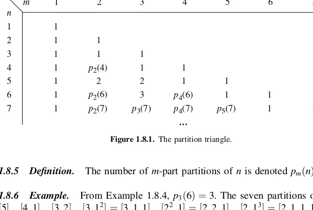
one is led to symmetric polynomials and, in Section 1.8, to partitions of n.

Elementary symmetric functions and their association with power sums lie at the

Combinatorics,Second Edition, by Russell Merris. ISBN 0-471-26296-X #2003 John Wiley & Sons, Inc.

(15)

heart of Section 1.9. The final section of the chapter is an optional introduction to algorithms, the flavor of which can be sampled by venturing only as far as Algorithm 1.10.3. Those desiring not less but more attention to algorithms can find it in Appendix A2.

1.1. THE FUNDAMENTAL COUNTING PRINCIPLE

How many different four-letter words, including nonsense words, can be produced by rearranging the letters in LUCK? In the absence of a more inspired approach, there is always the brute-force strategy: Make a systematic list.

Once we become convinced that Fig. 1.1.1 accounts for every possible rearran-gement and that no ‘‘word’’ is listed twice, the solution is obtained by counting the 24 words on the list.

While finding the brute-force strategy was effortless, implementing it required some work. Such an approach may be fine for an isolated problem, thelikeof which one does not expect to see again. But, just for the sake of argument, imagine your-self in the situation of having to solve a great many thinly disguised variations of this same problem. In that case, it would make sense to invest some effort in finding a strategy that requires less work to implement. Among the most powerful tools in this regard is the following commonsense principle.

1.1.1 Fundamental Counting Principle. Consider a (finite) sequence of deci-sions. Suppose the number of choices for each individual decision is independent of decisions made previously in the sequence. Then the number of ways to make the whole sequence of decisions is the product of these numbers of choices.

To state the principle symbolically, supposeciis the number of choices for deci-sion i. If, for 1i<n, ciþ1 does not depend on which choices are made in

LUCK LUKC LCUK LCKU LKUC LKCU

ULCK ULKC UCLK UCKL UKLC UKCL

CLUK CLKU CULK CUKL CKLU CKUL

KLUC KLCU KULC KUCL KCLU KCUL

(16)

decisions 1;. . .; i, then the number of different ways to make the sequence of decisions isc1c2 cn.

Let’s apply this principle to the word problem we just solved. Imagine yourself in the midst of making the brute-force list. Writing down one of the words involves a sequence of four decisions. Decision 1 is which of the four letters to write first, so

c1 ¼4. (It is no accident that Fig. 1.1.1 consists of four rows!) For each way of

making decision 1, there arec2¼3 choices for decision 2, namely which letter

to write second. Notice that the specific letters comprising these three choices

depend on how decision 1 was made, but theirnumberdoes not. That is what is

meant by the number of choices for decision 2 being independent of how the pre-vious decision is made. Of course,c3¼2, but what aboutc4? Facing no alternative, is it correct to say there is ‘‘no choice’’ for the last decision? If that were literally

true, then c4 would be zero. In fact, c4¼1. So, by the fundamental counting

principle, the number of ways to make the sequence of decisions, i.e., the number of words on the final list, is

c1c2c3c4¼4321:

The productn_ðn1Þ ðn2Þ 21 is commonly written n! and

readn-factorial: The number of four-letter words that can be made up by rearrang-ing the letters in the word LUCK is 4!¼24.

What if the word had been LUCKY? The number of five-letter words that can be

produced by rearranging the letters of the word LUCKY is 5!¼120. A systematic

list might consist of five rows each containing 4!¼24 words.

Suppose the word had been LOOT? How many four-letter words, including non-sense words, can be constructed by rearranging the letters in LOOT? Why not apply the fundamental counting principle? Once again, imagine yourself in the midst of making a brute-force list. Writing down one of the words involves a sequence of four decisions. Decision 1 is which of the three letters L, O, or T to write first. This time,c1¼3. But, what aboutc2? In this case, the number of choices for deci-sion 2 depends on how decideci-sion 1 was made! If, e.g.,Lwere chosen to be the first letter, then there would be two choices for the second letter, namely O or T. If, how-ever, O were chosen first, then there would be three choices for the second decision, L, (the second) O, or T. Do we takec2¼2 orc2¼3? The answer is thatthe

funda-mental counting principle does not apply to this problem (at least not directly).

The fundamental counting principle appliesonlywhen thenumberof choices for

decisioni_þ1 isindependentof how the previousidecisions are made.

To enumerate all possible rearrangements of the letters in LOOT, begin by dis-tinguishing the two O’s. maybe write the word as LOoT. Applying the fundamental counting principle, we find that there are 4!¼24 different-lookingfour-letter words that can be made up from L, O, o, and T.

*_{The exclamation mark is used, not for emphasis, but because it is a convenient symbol common to most}

(17)

Among the words in Fig. 1.1.2 are pairs like OLoT and oLOT, which look dif-ferent only because the two O’s have been distinguished. In fact, every word in the list occurs twice, once with ‘‘big O’’ coming before ‘‘little o’’, and once the other way around. Evidently, the number of different words (with indistinguishable O’s) that can be produced from the letters in LOOT is not 4! but 4!=2¼12.

What about TOOT? First write it as TOot. Deduce that in any list of all possible rearrangements of the letters T, O, o, and t, there would be 4!¼24 different-look-ing words. Dividdifferent-look-ing by 2 makes up for the fact that two of the letters are O’s. Divid-ing by 2 again makes up for the two T’s. The result, 24=ð22_{Þ ¼}6, is the number of different words that can be made up by rearranging the letters in TOOT. Here they are

TTOO TOTO TOOT OTTO OTOT OOTT

All right, what if the word had been LULL? How many words can be produced by rearranging the letters in LULL? Is it too early to guess a pattern? Could the number we’re looking for be 4!=3¼8? No. It is easy to see that the correct answer must be 4. Once the position of the letter U is known, the word is completely deter-mined. Every other position is filled with an L. A complete list is ULLL, LULL, LLUL, LLLU.

To find out why 4!/3 is wrong, let’s proceed as we did before. Begin by distin-guishing the three L’s, say L1, L2, and L3. There are 4! different-looking words that can be made up by rearranging the four letters L1, L2, L3, and U. If we were to make a list of these 24 words and then erase all the subscripts, how many times would, say, LLLU appear? The answer to this question can be obtained from the funda-mental counting principle! There are three decisions: decision 1 has three choices, namely which of the three L’s to write first. There are two choices for decision 2 (which of the two remaining L’s to write second) and one choice for the third deci-sion, which L to put last. Once the subscripts are erased, LLLU would appear 3!

times on the list. We should divide 4!_¼24, not by 3, but by 3!_¼6. Indeed,

4!=3!_¼4 is the correct answer.

Whoops! if the answer corresponding to LULL is 4!/3!, why didn’t we get 4!/2!

for the answer to LOOT? In fact, we did: 2!¼2.

Are you ready for MISSISSIPPI? It’s the same problem! If the letters were all different, the answer would be 11!. Dividing 11! by 4! makes up for the fact that there are four I’s. Dividing the quotient by another 4! compensates for the four S’s.

(18)

Dividing that quotient by 2! makes up for the two P’s. In fact, no harm is done if that quotient is divided by 1!¼1 in honor of the single M. The result is

11!

4!4!2!1!¼34;650:

(Confirm the arithmetic.) The 11 letters in MISSISSIPPI can be (re)arranged in 34,650 different ways.*

There is a special notation that summarizes the solution to what we might call the ‘‘MISSISSIPPI problem.’’

1.1.2 Definition. Themultinomial coefficient

n r1;r2;. . .;rk

¼ n!

r1!r2! rk! ;

wherer1þr2þ þrk¼n.

So, ‘‘multinomial coefficient’’ is aname for the answer to the question, how

manyn-letter ‘‘words’’ can be assembled using r1 copies of one letter, r2 copies of a second (different) letter, r3 copies of a third letter,. . .; and rk copies of a

kth letter?

1.1.3 Example. After cancellation,

9 4;3;1;1

¼9₄87654321 32132111

¼9875¼2520:

Therefore, 2520 different words can be manufactured by rearranging the nine letters

in the word SASSAFRAS. &

In real-life applications, the words need not be assembled from the English

alphabet. Consider, e.g., POSTNET{ barcodes commonly attached to U.S. mail

by the Postal Service. In this scheme, various numerical delivery codeszare repre-sented by ‘‘words’’ whose letters, orbits, come from the alphabetn; o. Correspond-ing, e.g., to a ZIP_þ4 code is a 52-bit barcode that begins and ends with . The 50-bit middle part is partitioned into ten 5-50-bit zones. The first nine of these zones are for the digits that comprise the ZIP_þ4 code. The last zone accommodates aparity

*_{This number is roughly equal to the number of members of the Mathematical Association of America}

(MAA), the largest professional organization for mathematicians in the United States. {_{Postal Numeric Encoding Technique.}

(19)

checkdigit, chosen so that the sum of all ten digits is a multiple of 10. Finally, each digit is represented by one of the 5-bit barcodes in Fig. 1.1.3. Consider, e.g., the ZIP

þ4 code 20090-0973, for the Mathematical Association of America. Because the

sum of these digits is 30, the parity check digit is 0. The corresponding 52-bit word can be found in Fig. 1.1.4.

20090-0973 Figure 1.1.4

We conclude this section with another application of the fundamental counting principle.

1.1.4 Example. Suppose you wanted to determine the number of positive

integers that exactly divide n_¼12. That isn’t much of a problem; there are six

of them, namely, 1, 2, 3, 4, 6, and 12. What about the analogous problem for

n_¼360 or for n_¼360;000? Solving even the first of these by brute-force list

making would be a lot of work. Having already found another strategy whose implementation requires a lot less work, let’s take advantage of it.

Consider 360_¼23₃2_{5, for example. If 360}_¼_dq _{for positive integers} _d

andq, then, by the uniqueness part of thefundamental theorem of arithmetic, the prime factors of d, together with the prime factors of q, are precisely the prime factors of 360, multiplicities included. It follows that the prime factorization ofd

must be of the formd_¼2a 3b

5c_{, where 0}

a3, 0b2, and 0c1.

Evidently, there are four choices fora(namely 0, 1, 2, or 3), three choices forb, and

two choices forc. So, the number of possibiled’s is 432_¼24. &

1.1. EXERCISES

1 The Hawaiian alphabet consists of 12 letters, the vowels a, e, i,o,u and the consonantsh,k,l,m,n,p,w.

(a) Show that 20,736 different 4-letter ‘‘words’’ could be constructed using the 12-letter Hawaiian alphabet.

0 =

5 =

1 =

6 =

2 =

7 =

3 =

8 =

4 =

(20)

(b) Show that 456,976 different 4-letter ‘‘words’’ could be produced using the 26-letter English alphabet.*

(c) How many four-letter ‘‘words’’ can be assembled using the Hawaiian

alphabet if the second and last letters are vowels and the other 2 are consonants?

(d) How many four-letter ‘‘words’’ can be produced from the Hawaiian

alphabet if the second and last letters are vowels but there are no restrictions on the other 2 letters?

3 One brand of electric garage door opener permits the owner to select his or her

own electronic ‘‘combination’’ by setting six different switches either in the ‘‘up’’ or the ‘‘down’’ position. How many different combinations are possible?

4 One generation back you have two ancestors, your (biological) parents. Two

generations back you have four ancestors, your grandparents. Estimating 210_as

103_{, approximately how many ancestors do you have}

(a) 20 generations back?

(b) 40 generations back?

(c) In round numbers, what do you estimate is the total population of the

planet?

(d) What’s wrong?

5 Make a list of all the ‘‘words’’ that can be made up by rearranging the letters in

(a) TO. (b) TOO. (c) TWO.

*_{Based on these calculations, might it be reasonable to expect Hawaiian words, on average, to be longer}

(21)

(d) 6

3;2;1

: (e) 6

1;3;2

. (f) 6

1;1;1;1;1;1

.

7 How many different ‘‘words’’ can be constructed by rearranging the letters in

(a) ALLELE? (b) BANANA? (c) PAPAYA?

(d) BUBBLE? (e) ALABAMA? (f) TENNESSEE?

(g) HALEAKALA? (h) KAMEHAMEHA? (i) MATHEMATICS?

8 Prove that

(a) 1þ2þ22_þ₂3_{þ þ}₂n_¼₂nþ1_1.

(b) 11!þ22!þ33!þ þnn!¼ ðn_þ1Þ!1.

(c) ð2n_Þ!=2n _{is an integer.}

9 Show that the barcodes in Fig. 1.1.3 comprise all possible five-letter words

consisting of two ’s and three ’s.

10 Explain how the following barcodes fail the POSTNET standard:

(a)

(b)

(c)

11 ‘‘Read’’ the ZIP_þ4 Code

(a)

(b)

12 Given that the first nine zones correspond to the ZIP_þ4 delivery code

94542-2520, determine the parity check digit and the two ‘‘hidden digits’’ in the 62-bit DPBC

(Hint:Do you need to be told that the parity check digit is last?)

13 Write out the 52-bit POSTNET barcode for 20742-2461, the ZIP_þ4 code at

the University of Maryland used by the Association for Women in Mathematics.

14 Write out all 24 divisors of 360. (See Example 1.1.4.)

15 Compute the number of positive integer divisors of

(a) 210_. _(b) ₁₀10_. _(c) ₁₂10_. _(d) ₃₁10_.

(22)

16 Prove that the positive integernhas an odd number of positive-integer divisors if and only if it is a perfect square.

17 LetD_¼fd1;d2;d3;d4g andR¼fr1;r2;r3;r4;r5;r6g. Compute the number

(a) of different functionsf : D_!R.

(b) of one-to-one functions f : D_!R.

18 The latest automobile license plates issued by the California Department of

Motor Vehicles begin with a single numeric digit, followed by three letters, followed by three more digits. How many different license ‘‘numbers’’ are available using this scheme?

19 One brand of padlocks uses combinations consisting of three (not necessarily

different) numbers chosen from 0;_f 1;2;. . .;39_g. If it takes five seconds to ‘‘dial in’’ a three-number combination, how long would it take to try all possible combinations?

20 TheInternational Standard Book Number(ISBN) is a 10-digit numerical code for identifying books. The groupings of the digits (by means of hyphens) varies from one book to another. The first grouping indicates where the book was published. In ISBN 0-88175-083-2, the zero shows that the book was published in the English-speaking world. The code for the Netherlands is ‘‘90’’ as, e.g., in ISBN 90-5699-078-0. Like POSTNET, ISBN employs a check digit scheme. The first nine digits (ignoring hyphens) are multiplied, respectively, by 10, 9, 8;. . .;2, and the resulting products summed to obtainS. In 0-88175-083-2, e.g.,

S_¼100_þ98_þ88_þ71_þ67_þ55_þ40 þ38þ23¼240:

The last (check) digit,L, is chosen so thatS_þLis a multiple of 11. (In our

example,L_¼2 andS_þL_¼242_¼1122.)

(a) Show that, whenSis divided by 11, the quotientQand remainderRsatisfy

S_¼11Q_þR.

(b) Show that L_¼11R. (WhenR_¼1, the check digit is X.)

(c) What is the value of the check digit,L, in ISBN 0-534-95154-L?

(d) Unlike POSTNET, the more sophisticated ISBN system can not

only detect common errors, it can sometimes ‘‘correct’’ them. Suppose, e.g., that a single digit is wrong in ISBN 90-5599-078-0. Assuming the check digit is correct, can you identify the position of the erroneous digit?

(e) Now that you know the position of the (single) erroneous digit in part (d), can you recover the correct ISBN?

(f) What if it were expected that exactly two digits were wrong in part (d).

(23)

21 A total of 9!¼362;880 different nine-letter ‘‘words’’ can be produced by rearranging the letters in FULBRIGHT. Of these, how many contain the four-letter sequence GRIT?

22 In how many different ways can eight coins be arranged on an 88

checkerboard so that no two coins lie in the same row or column?

23 If A is a finite set, its cardinality, o_ðA_Þ, is the number of elements in A. Compute

(a) o_ðA_Þwhen A is the set consisting of all five-digit integers, each digit of which is 1, 2, or 3.

(b) o_ðB_Þ, where B_¼_fx₂A : each of 1;2;and 3 is among the digits of x_g

andAis the set in part (a).

1.2. PASCAL’S TRIANGLE

Mathematics is the art of giving the same name to different things.

— Henri Poincare´ (1854–1912)

In how many different ways can anr-element subset be chosen from ann-element

setS? Denote the number byC_ðn;r_Þ. Pronounced ‘‘n-choose-r’’,C_ðn;r_Þ is just a name for the answer. Let’s find the number represented by this name.

Some facts aboutC_ðn;r_Þare clear right away, e.g., the nature of the elements of

Sis immaterial. All that matters is that there arenof them. Because the only way to choose ann-element subset fromS is to choose all of its elements,C_ðn;n_{Þ ¼}1. Having n single elements, S has n single-element subsets, i.e., C_ðn;1Þ ¼n. For essentially the same reason, C_ðn;n1Þ ¼n: A subset of S that contains all but one element is uniquely determined by the one element that is left out. Indeed, this idea has a nice generalization. A subset ofS that contains all butrelements

is uniquely determined by the r elements that are left out. This natural

one-to-one correspondence between subsets and their complements yields the following

symmetry property:

C_ðn;nr_{Þ ¼}C_ðn;r_Þ:

(24)

A;B

f g $_fC;D;E_g; _fB;D_{g $}_fA;C;E_g;

A;C

f g $_fB;D;E_g; _fB;E_{g $}_fA;C;D_g;

A;D

f g $_fB;C;E_g; _fC;D_{g $}_fA;B;E_g;

A;E

f g $_fB;C;D_g; _fC;E_{g $}_fA;B;D_g;

B;C

f g $_fA;D;E_g; _fD;E_{g $}_fA;B;C_g:

By counting these pairs, we find thatC_ð5;2_{Þ ¼}C_ð5;3_{Þ ¼}10. &

A special case of symmetry isC_ðn;0_{Þ ¼}C_ðn;n_{Þ ¼}1. Givennobjects, there is just one way to reject all of them and, hence, just one way to choose none of them.

What ifn_¼0? How many ways are there to choose no elements from the empty

set? To avoid a deep philosophical discussion, let us simply adopt as a convention thatC_ð0;0Þ ¼1.

A less obvious fact about choosing these numbers is the following.

1.2.2 Theorem (Pascal’s Relation). If1rn, then

C_ðn_þ1;r_{Þ ¼}C_ðn;r1Þ þC_ðn;r_Þ: ð1:1Þ

Together with Example 1.2.1, Pascal’s relation implies, e.g., that C_ð6;3_{Þ ¼}

C_ð5;2Þ þC_ð5;3Þ ¼20.

Proof. Consider theðn_þ1Þ-element set_fx1;x2;. . .;xn;y_g. Itsr-element subsets

can be partitioned into two families, those that contain y and those that do not.

To count the subsets that containy, simply observe that the remaining r1

ele-ments can be chosen from fx1;x2;. . .;xng in Cðn;r1Þ ways. The r-element

subsets that do not contain y are precisely the r-element subsets of

x1;x2;. . .;xn

f g, of which there areC_ðn;r_Þ. &

The proof of Theorem 1.2.2 used another self-evident fact that is worth men-tioning explicitly. (A much deeper extension of this result will be discussed in Chapter 2.)

1.2.3 The Second Counting Principle. If a set can be expressed as the disjoint union of two (or more) subsets, then the number of elements in the set is the sum of the numbers of elements in the subsets.

So far, we have been viewingC_ðn;r_Þas a single number. There are some advan-tages to looking at these choosing numbers collectively, as in Fig. 1.2.1. The trian-gular shape of this array is a consequence of not bothering to write 0¼C_ðn;r_Þ,

(25)

Given the fourth row of the array (corresponding ton_¼3), we can use Pascal’s relation to computeC_ð4;2Þ ¼C_ð3;1Þ þC_ð3;2Þ ¼3þ3¼6. Similarly,C_ð6;4Þ ¼

C_ð6;2Þ ¼C_ð5;1Þ þC_ð5;2Þ ¼5þ10¼15. Continuing in this way, one row at a time, we can complete as much of the array as we like.

Following Western tradition, we refer to the array in Fig. 1.2.3 as Pascal’s

triangle.*(Take care not to forget, e.g., thatC_ð6;3_{Þ ¼}20 appears, not in the third column of the sixth row, but in the fourth column of the seventh!)

Pascal’s triangle is the source of many interesting identities. One of these con-cerns the sum of the entries in each row:

1þ1¼2;

*_{After Blaise Pascal (1623–1662), who described it in the book}_{Traite´ du triangle arithme´tique}_{. Rumored}

to have been included in a lost mathematical work by Omar Khayyam (ca. 1050–1130), author of the

Rubaiyat, the triangle is also found in surviving works by the Arab astronomer al-Tusi (1265), the Chinese mathematician Chu Shih-Chieh (1303), and the Hindu writer Narayana Pandita (1365). The first European author to mention it was Petrus Apianus (1495–1552), who put it on the title page of his 1527 book,

(26)

and so on. Why should each row sum to a power of 2? In

two-element subsets, and so on. Evidently, the sum of the numbers in row n of

Pascal’s triangle is the total number of subsets of S (even when n_¼0 and

S_¼[_Þ. The empirical evidence from Equations (1.2) suggests that an n-element

set has a total of 2n_{subsets. How might one go about proving this conjecture?} One way to do it is by mathematical induction. There is, however, another approach that is both easier and more revealing. Imagine youself in the process of listing the subsets of S_¼fx1;x2;. . .;xng. Specifying a subset involves a sequence of decisions. Decision 1 is whether to includex1. There are two choices,

Yes or No. Decision 2, whether to put x2 into the subset, also has two choices.

Indeed, there are two choices for each of thendecisions. So, by the fundamental

counting principle,S has a total of 222_¼2n _subsets.

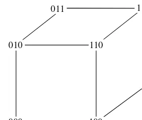
There is more. Suppose, for example, thatn_¼9. Consider the sequence of

deci-sions that produces the subsetfx2;x3;x6;x8g, a sequence that might be recorded as NYYNNYNYN. The first letter of this word corresponds toNo, as in ‘‘no tox1’’; the second letter corresponds toYes, as in ‘‘yes tox2’’; becausex3is in the subset, the third letter is Y; and so on for each of the nine letters. Similarly,fx1;x2;x3g cor-responds to the nine-leter word YYYNNNNNN. In general, there is a one-to-one correspondence between subsets of_fx1;x2;. . .;xng, andn-letter words assembled

from the alphabet _fN;Y_g. Moreover, in this correspondence, r-element subsets

correspond to words withrY’s and nrN’s.

We seem to have discovered a new way to think aboutC_ðn;r_Þ. It is the number

ofn-letter words that can be produced by (re)arrangingrY’s and nr N’s. This

interpretation can be verified directly. Ann-letter word consists ofnspaces, or loca-tions, occupied by letters. Each of the words we are discussing is completely

deter-mined once therlocations of the Y’s have been chosen (the remainingnrspaces

(27)

The significance of this new perspective is that we know how to count the

num-ber ofn-letter words withrY’s and nrN’s. That’s the MISSISSIPPI problem!

The answer is multinomial coefficient n

r;nr

It is common in the mathematical literature to writen r justification being that the information conveyed by ‘‘nr’’ is redundant. It can be

computed fromnandr. The same thing could, of course, be said aboutany

multi-nomial coefficient. The last number in the second row is always redundant. So, that particular argument is not especially compelling. The honest reason for writingn

r

combinatorial definition:n-choose-ris the number of ways to chooserthings from a collection ofnthings. The alternative, what we might call thealgebraic definition, is

C_ðn;r_{Þ ¼} n! r!_ðnr_Þ!:

Don’t make the mistake of asuming, just because it is more familiar, that the algebraic definition will always be easiest. (Try giving an algebraic proof of the identityPn_r_¼₀ C_ðn;r_{Þ ¼}2n_{.) Some applications are easier to approach using} alge-braic methods, while the combinatorial definition is easier for others. Only by becoming familiar with both will you be in a position to choose the easiest approach in every situation!

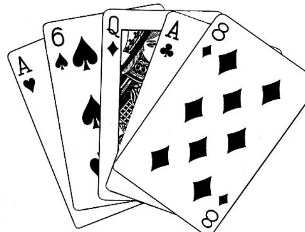
1.2.4 Example. In the basic version of poker, each player is dealt five cards (as in Fig. 1.2.4) from a standard 52-card deck (no joker). How many different five-card

poker hands are there? Because someone (in a fair game it might beLady Luck)

chooses five cards from the deck, the answer isC_ð52;5_Þ. The ways to find the num-ber behind this name are: (1) Make an exhaustive list of all possible hands, (2) work out 52 rows of Pascal’s triangle, or (3) use the algebraic definition

(28)

1.2.5 Example. The game of bridge uses the same 52 cards as poker.* The number of different 13-card bridge hands is

C_ð52;13_{Þ ¼} 52! 13!39!

¼5251 4039!

13!39!

¼5251 40

13! ;

about 635,000,000,000. &

It may surprise you to learn thatC_ð52;13_Þis so much larger thanC_ð52;5_Þ. On the other hand, it does seem clear from Fig. 1.2.3 that the numbers in each row of Pascal’s triangle increase, from left to right, up to the middle of the row and then decrease from the middle to the right-hand end. Rows for which this property holds are said to beunimodal.

1.2.6 Theorem. The rows of Pascal’s triangle are unimodal.

(29)

Proof. Ifn>2r_þ1, the ratio

3 Write out rows 7 through 10 of Pascal’s triangle and confirm that the sum of

the numbers in the 10th row is 210 _¼_1024.

6 Poker is sometimes played with a joker. How many different five-card poker

hands can be ‘‘chosen’’ from a deck of 53 cards?

7 Phrobana is a game played with a deck of 48 cards (no aces). How many

different 12-card phrobana hands are there?

8 Give the inductive proof that ann-element set has 2n _subsets.

(30)

(a) using algebraic arguments.

(b) using combinatorial arguments.

10 Supposen,k, andrare integers that satisfynkr0 andk>0. Prove

that

(a) C_ðn;k_ÞC_ðk;r_{Þ ¼}C_ðn;r_ÞC_ðnr;kr_Þ.

(b) C_ðn;k_ÞC_ðk;r_{Þ ¼}C_ðn;kr_ÞC_ðnk_þr;r_Þ.

(c) Pn_j_¼₀ C_ðn;j_ÞC_ðj;r_{Þ ¼}C_ðn;r_Þ2nr_.

(d) Pn_j_¼_kð1ÞjþkC_ðn;j_{Þ ¼}C_ðn1;k1Þ.

11 Prove that Pnr_¼0 Cðn;rÞ 2

¼P2ns_¼0 Cð2n;sÞ.

12 Prove thatC_ð2n;n_Þ,n>0, is always even.

13 Probably first studied by Leonhard Euler (1707–1783), theCatalan sequence*

1, 1, 2, 5, 14, 42, 132, 429, 1430, 4862;. . . is defined by cn¼Cð2n;nÞ= ðn_þ1_Þ,n0. Confirm that the Catalan numbers satisfy

(a) c2¼2c1. (b) c3¼3c2c1.

(c) c4¼4c33c2. (d) c5¼5c46c3þc2.

(e) c6¼6c510c4þ4c3. (f) c7¼7c615c5þ10c4c3.

(g) Speculate about the general form of these equations.

(h) Prove or disprove your speculations from part (g).

14 Show that the Catalan numbers (Exercise 13) satisfy

(a) cn¼Cð2n1;n1Þ Cð2n1;nþ1Þ.

(b) cn¼Cð2n;nÞ Cð2n;n1Þ.

(c) cnþ1¼4_nn_þþ₂2cn.

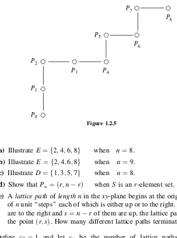
15 One way to illustrate anr-element subsetSof 1;_f 2;. . .;n_gis this: LetP0 be the origin of thexy-plane. Settingx0 ¼y0¼0, define

Pk¼ ðxk;ykÞ ¼ ð

xk1þ1;yk1Þ if k2S; ðxk1;yk1þ1Þ if k62S:

Finally, connect successive points by unit segments (either horizontal or vertical) to form a ‘‘path’’. Figure 1.2.5 illustrates the path corresponding to

S_¼_f3;4;6;8_gandn_¼8.

*_{Euler was so prolific that more than one topic has come to be named for the first person to work on it}_after

(31)

P0 P1 P2

P₃ P₄

P₆

P₈ P7

P₅

Figure 1.2.5

(a) IllustrateE_¼_f2;4;6;8_g when n_¼8.

(b) Illustrate E_¼_f2;4;6;8_g when n_¼9.

(c) IllustrateD_¼_f1;3;5;7_g when n_¼8.

(d) Show that Pn¼ ðr;nrÞ when Sis anr-element set.

(e) Alattice pathoflength nin thexy-plane begins at the origin and consists ofnunit ‘‘steps’’ each of which is either up or to the right. Ifrof the steps are to the right ands_¼nrof them are up, the lattice path terminates at the pointðr;s_Þ. How many different lattice paths terminate atðr;s_Þ?

16 Define c0¼1 and let cn be the number of lattice paths of length 2n

(Exercise 15) that terminate at ðn;n_Þ and never rise above the line y_¼x, i.e., such thatxkykfor each pointPk¼ðxk;ykÞ. Show that

(a) c1¼1;c2¼2, andc3¼5.

(b) cn_þ1 ¼Pnr_¼0 crcnr. (Hint:Lattice paths ‘‘touch’’ the liney¼xfor the last time at the point_ðn;n_Þ. Count those whose next-to-last touch is at the point_ðr;r_Þ).

(c) cnis the nth Catalan number of Exercises 13–14,n1.

17 LetXandY be disjoint sets containingnandmelements, respectively. In how

many different ways can anðr_þs_Þ-element subsetZbe chosen fromX_[Y if

rof its elements must come fromX andsof them fromY?

18 Packing for a vacation, a young man decides to take 3 long-sleeve shirts,

(32)

n r 0 1 2 3 4 5 6 7

0 C(0,0)

1 C(1,0) C(1,1)

2 C(2,0) C(2,1) C(2,2)

3 C(3,0) C(3,1) C(3,2)

+ C(3,3)

4 C(4,0) C(4,1)

+ C(4,2) C(4,3) C(4,4)

5 C(5,0)

+ C(5,1) C(5,2) C(5,3) C(5,4) C(5,5)

6 C(6,0) C(6,1) C(6,2) C(6,3) C(6,4) C(6,5) C(6,6)

7 C(7,0) C(7,1) C(7,2) C(7,3) C(7,4) C(7,5) C(7,6) C(7,7)

. . .

Figure 1.2.6

19 Supposenis a positive integer and letk_{¼ b}n=2c, the greatest integer not larger thann=2. Define

Fn ¼Cðn;0Þ þCðn1;1Þ þCðn2;2Þ þ þCðnk;kÞ:

Starting withn_¼0, the sequencef gFn is

1;1;2;3;5;8;13;. . .;

where, e.g., the 7th number in the sequence, F6¼13, is computed by

summing theboldfacenumbers in Fig. 1.2.6.*

(a) ComputeF7 directly from the definition.

(b) Prove the recurrence Fnþ2¼Fnþ1þFn,n0.

(c) ComputeF7using part (b) and the initial fragment of the sequence given

above.

(d) Prove thatPn_i_¼₀ Fi¼Fnþ21.

20 C. A. Tovey used the Fibonacci sequence (Exercise 19) to prove that infinitely

many pairs_ðn;k_Þsolve the equationC_ðn;k_{Þ ¼}C_ðn1;k_þ1_Þ. The first pair is

C_ð2;0_{Þ ¼}C_ð1;1_Þ. Find the second. (Hint: n<20. Your solution need not make use of the Fibonacci sequence.)

21 The Buda side of the Danube is hilly and suburban while the Pest side is flat

and urban. In short, Budapest is a divided city. Following the creation of a new commission on culture, suppose 6 candidates from Pest and 4 from Buda volunteer to serve. In how many ways can the mayor choose a 5-member commission.

*_{It was the French number theorist Franc¸ois E´douard Anatole Lucas (1842–1891) who named these}

(33)

(a) from the 10 candidates?

(b) if proportional representation dictates that 3 members come from Pest and 2 from Buda?

22 H. B. Mann and D. Shanks discovered a criterion for primality in terms of

Pascal’s triangle: Shift each of then_þ1 entries in rown to the right so that they begin in column 2n. Circle the entries in rown that are multiples of n.

Thenris prime if and only if all the entries in columnr have been circled.

Columns 0–11 are shown in Fig. 1.2.7. Continue the figure down to row 9 and out to column 20.

23 The superintendent of the Hardluck Elementary School District suggests that

the Board of Education meet a $5 million budget deficit by raising average class sizes, from 30 to 36 students, a 20% increase. A district teacher objects,

pointing out that if the proposal is adopted, the potential for a pair of

classmates to get into trouble will increase by 45%. What is the teacher talking about?

24 Strictly speaking, Theorem 1.2.6 establishes only half of the unimodality

property. Prove the other half.

25 If n and r are nonnegative integers and x is an indeterminate, define

K_ðn;r_{Þ ¼ ð}1_þx_Þnxr.

(a) Show thatK_ðn_þ1;r_{Þ ¼}K_ðn;r_{Þ þ}K_ðn;r_þ1_Þ.

(b) Compare and contrast the identity in part (a) with Pascal’s relation.

(c) Since part (a) is a polynomial identity, it holds when numbers are

substituted for x. Let k_ðn;r_Þ be the value of K_ðn;r_Þ when x_¼2 and exhibit the numbers k_ðn;r_Þ, 0n, r4, in a 55 array, the rows of which are indexed bynand the columns byr. (Hint:Visually confirm that

(34)

26 LetS be ann-element set, wheren1. IfAis a subset ofS, denote byo_ðA_Þ

thecardinalityof (number of elements in)A. Say thatAis odd (even) ifo_ðA_Þis odd (even). Prove that the number of odd subsets ofSis equal to the number of its even subsets.

27 Show that there are exactly seven different ways to factor n_¼63;000 as a

product of two relatively prime integers, each greater than one.

28 Supposen_¼pa1₁pa2₂ par

r, wherep1;p2;. . .;pr are distinct primes. Prove that

there are exactly 2r1_{1 different ways to factor} _n _{as a product of two}

relatively prime integers, each greater than one.

*1.3. ELEMENTARY PROBABILITY

The theory of probabilities is basically only common sense reduced to calculation; it makes us appreciate with precision what reasonable minds feel by a kind of instinct, often being unable to account for it.. . . It is remarkable that [this] science, which began with the consideration of games of chance, should have become the most impor-tant object of human knowledge.

— Pierre Simon, Marquis de Laplace (1749–1827)

Elementary probability theory begins with the consideration of D equally likely

‘‘events’’ (or ‘‘outcomes’’). If N of these are ‘‘noteworthy’’, then the probability

of a noteworthy event is the fraction N=D. Maybe a brown paper bag contains a

dozen jelly beans, say, 1 red, 2 orange, 2 blue, 3 green, and 4 purple. If a jelly bean is chosen at random from the bag, the probability that it will be blue is

2

12¼

1

6; the probability that it will be green is 3

12¼

1

4; the probability that it will be blue or green is ð2þ3Þ=12¼ 5

12; and the probability that it will be blue and green is 0

12¼0.

Dice are commonly associated with games of chance. In a dice game, one is typically interested only in the numbers that rise to the top. If a single die is rolled, there are just six outcomes; if the die is ‘‘fair’’, each of them is equally likely. In computing the probability, say, of rolling a number greater than 4 with a single fair

die, the denominator isD_¼6. Since there areN_¼2 noteworthy outcomes, namely

5 and 6, the probability we want isP_¼2₆_¼1₃.

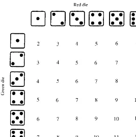
The situation is more complicated when two dice are rolled. If all we care about is their sum, then there are 11 possible outcomes, anything from 2 to 12. But, the probability of rolling a sum, say, of 7 is not 1

11because these 11 outcomes are not

(35)

one sees that there are six ways the dice can sum to 7, namely, a green 1 and a red 6, a green 2 and a red 5, a green 3 and a red 4, and so on. So, the probability of rolling a (sum of ) 7 is not₁₁1 but₃₆6 ¼1

6:

1.3.1 Example. Denote by P_ðn_Þ the probability of rolling (a sum of ) n with

two fair dice. Using Fig. 1.3.1, it is easy to see that P_ð2_{Þ ¼} 1

36¼Pð12Þ,

P_ð3_{Þ ¼} 2

36¼

1

18¼Pð11Þ, Pð4Þ ¼

3

36¼

1

12¼Pð10Þ, and so on. What about Pð1Þ? Since 1 is not among the outcomes,P_ð1_{Þ ¼} 0

36¼0. In fact, ifPis some probability

(any probability at all), then 0P1. &

1.3.2 Example. A popular game at charity fundraisers is Chuck-a-Luck. The apparatus for the game consists of three dice housed in an hourglass-shaped cage. Once the patrons have placed their bets, the operator turns the cage and the dice roll to the bottom. If none of the dice comes up 1, the bets are lost. Otherwise, the operator matches, doubles, or triples each wager depending on the number of ‘‘aces’’ (1’s) showing on the three dice.

Let’s compute probabilities for various numbers of 1’s. By the fundamental counting principle, there are 63 _¼_{216 possible outcomes (all of which are equally}

(36)

likely if the dice are fair). Of these 216 outcomes, only one consists of three 1’s. Thus, the probability that the bets will have to be tripled is 1

216.

In how many ways can two 1’s come up? Think of it as a sequence of two deci-sions. The first is which die should produce a number different from 1. The second is what number should appear on that die. There are three choices for the first

deci-sion and five for the second. So, there are 35¼15 ways for the three dice to

produce exactly two 1’s. The probability that the bets will have to be doubled is₂₁₆15. What about a single ace? This case can be approached as a sequence of three decisions. Decision 1 is which die should produce the 1 (three choices). The second decision is what number should appear on the second die (five choices, anything but 1). The third decision is the number on the third die (also five choices). Evidently,

there are 355_¼75 ways to get exactly one ace. So far, we have accounted for

1_þ15_þ75_¼91 of the 216 possible outcomes. (In other words, the probability of gettingat leastone ace is 91

216.) In the remaining 21691¼125 outcomes, three

are no 1’s at all. These results are tabulated in Fig. 1.3.2. &

Some things, like determining which team kicks off to start a football game, are decided by tossing a coin. A fair coin is one in which each of the two possible out-comes, heads or tails, is equally likely. When a fair coin is tossed, the probability that it will come up heads is1

2.

Suppose four (fair) coins are tossed. What is the probability that half of them will be heads and half tails? Is it obvious that the answer is3

8? Once again, Lady

Luck has a sequence of decisions to make, this time four of them. Since there are two choices for each decision,D_¼24_{. With the noteworthies in}_boldface_{, these 16} outcomes are arrayed in Fig. 1.3.3. By inspection,N_¼6, so the probability we seek is 6

16¼38.

HHHH HTHH THHH TTHH

HHHT HTHT THHT T T H T

HHTH HTTH THTH T T T H

HHTT H T T T T H T T T T T T

Figure 1.3.3

1.3.3 Example. If 10 (fair) coins are tossed, what is the probability that half of them will be heads and half tails? Ten decisions, each with two choices, yields

D_¼210_¼_{1024. To compute the numerator, imagine a systematic list analogous}

to Fig. 1.3.3. In the case of 10 coins, the noteworthy outcomes correspond to

Number of 1’s 0 1 2 3

Probability 125 75 15 1

216 216 216 216

(37)

10-letter ‘‘words’’ with fiveH’s and fiveT’s, soN_¼₅10_;₅_{Þ ¼}C_ð10;5_{Þ ¼}252, and the desired probability is 252

1024¼_ 0:246. More generally, if n coins are tossed, the probability that exactlyr of them will come up heads isC_ðn;r_Þ=2n_.

What about the probability thatat most rof them will come up heads? That’s

easy enough: P_¼N=2n_{, where} _N_¼_N_ð_n_;_r_{Þ ¼}_C_ð_n_;₀_{Þ þ}_C_ð_n_;₁_{Þ þ þ}_C_ð_n_;_r_Þ is the number ofn-letter words that can be assembled from the alphabet_fH;T_g

and that contain at mostr H’s. &

Here is a different kind of problem: Suppose two fair coins are tossed, say a dime and a quarter. If you are told (only) that one of them is heads, what is the probability that the other one is also heads? (Don’t just guess, think about it.)

May we assume, without loss of generality, that the dime is heads? If so, because the quarter has a head of its own, so to speak, the answer should be1

2. To see why this is wrong, consider the equally likely outcomes when two fair coins are tossed, namely,HH,HT,TH, andTT. If all we know is that one (at least) of the coins is heads, thenTTis eliminated. Since the remaining three possibilities are still equally likely,D_¼3, and the answer is 1

3.

There are two ‘‘morals’’ here. One is that the most reliable guide to navigating probability theory is equal likelihood. The other is that finding a correct answer often depends on having a precise understanding of the question, and that requires precise language.

1.3.4 Definition. A nonempty finite setEof equally likely outcomes is called a

sample space. The number of elements inEis denotedo_ðE_Þ. For any subsetAofE, the probability ofAisP_ðA_{Þ ¼}o_ðA_Þ=o_ðE_Þ. If Bis a subset ofE, then P_ðAorB_{Þ ¼} P_ðA_[B_Þ, and P_ðAandB_{Þ ¼}P_ðA_\B_Þ.

In mathematical writing, an unqualified ‘‘or’’ is inclusive, as in ‘‘AorBor both’’.*

1.3.5 Theorem. Let E be a fixed but arbitrary sample space. If A and B are subsets of E, then

P_ðA orB_{Þ ¼}P_ðA_{Þ þ}P_ðB_ÞP_ðAandB_Þ:

Proof. The sumo_ðA_{Þ þ}o_ðB_Þcounts all the elements ofAand all the elements of

B. It even counts some elements twice, namely those inA_\B. Subtractingo_ðA_\B_Þ

compensates for this double counting and yields

o_ðA_[B_{Þ ¼}o_ðA_{Þ þ}o_ðB_Þo_ðA_\B_Þ:

(Notice that this formula generalizes the second counting principle; it is a special case of the even more general principle of inclusion and exclusion, to be

discussed in Chapter 2.) It remains to divide both sides by o_ðE_Þ and use

Definition 1.3.4.

&

(38)

1.3.6 Corollary. Let E be a fixed but arbitrary sample space. If A and B are subsets of E, then P_ðA or B_ÞP_ðA_{Þ þ}P_ðB_Þwith equality if and only if A and B are disjoint.

Proof. P_ðAandB_Þ¼0 if and only ifo_ðA_\B_Þ¼0 if and only ifA_\B_¼[. &

A special case of this corollary involves thecomplement,Ac_¼_fx₂E : x₆₂A_g. Since A_[Ac_¼E and A_\Ac_¼[,o_ðA_{Þ þ}o_ðAc_{Þ ¼}o_ðE_Þ. Dividing both sides of this equation byo_ðE_Þyields the useful identity

P_ðA_{Þ þ}P_ðAc_{Þ ¼}1:

1.3.7 Example. Suppose two fair dice are rolled, say a red one and a green one. What is the probability of rolling a 3 on the red die, call it a red 3, or a green 2?

Let’s abbreviate by setting R3¼red 3 and G2¼green 2 so that, e.g.,

P_ðR3Þ ¼1

6¼PðG2Þ.

Solution 1: When both dice are rolled, only one of the 62_¼_{36 equally likely}

outcomes corresponds to R3 and G2, so P_ðR3 andG2Þ ¼ 1

36. Thus, by Theorem

1.3.5,

P_ðR3 orG2_{Þ ¼}P_ðR3_{Þ þ}P_ðG2_ÞP_ðR3 andG2_Þ ¼1

6þ

1

6

1 36 ¼11

36:

Solution 2: Let Pc be the complementary probability that neither R3 nor G2

occurs. Then Pc¼N=D, where D¼36. The evaluation of N can be viewed in

terms of a sequence of two decisions. There are five choices for the ‘‘red’’ decision, anything but number 3, and five for the ‘‘green’’ one, anything but number 2. Hence,N_¼55¼25, and Pc¼25₃₆, so the probability we want is

P_ðR3 orG2Þ ¼1Pc¼11₃₆:

&

1.3.8 Example. Suppose a single (fair) die is rolled twice. What is the probabil-ity that the first roll is a 3 or the second roll is a 2? Solution:11

36. This problem is

equivalent to the one in Example 1.3.7. &

1.3.9 Example. Suppose a single (fair) die is rolled twice. What is the probabil-ity of getting a 3 or a 2?

Solution 1: Of the 66_¼36 equally likely outcomes, 44_¼16 involve