Jurnal Bina Praja 9 (1) (2017): 1-13
Jurnal Bina Praja
e-ISSN: 2503-3360 p-ISSN: 2085-4323
http://binaprajajournal.com
Determinants of Paddy Field Conversion
in Java 1995-2013
Wina Dwi Febrina
* Research and Development CenterNational Land Agency
Jl. H. Agus Salim No. 58, Menteng, Central Jakarta
Received: 25 November 2016; Accepted: 24 March 2017; Published online: 31 May 2017
DOI: 10.21787/jbp.09.2017.1-13
Abstract
Java is the biggest rice supplier with the largest paddy field compared to other islands in Indonesia. On the other side, economic growth needs more and more land for infrastructure growth. It was suggested that the growth would convert paddy field in Java to non-agriculture use. This paper reports the growth of land conversion, especially from paddy field to other utilization, in Java Island using panel data (provincial data 1995-2013). The data then treated as the dependent variable in the regression analysis for determining the factors that are significantly influential. The relative strengths of the influential factors are then compared using the concept of elasticity. It is found that farmers term of trade and GDP of manufacturing industries sectors significantly influence the land conversion. Meanwhile, the size of the population and the size of medium and large companies of manufacturing industries do not significantly influence the land conversion.
Keywords: Paddy Field Conversion, Determinant Factors
I. Introduction
A land is a resource that physically cannot be produced so that the supply of land is limited. On the other side, the high demand for land for a variety of activities tend to exceed the supply of available land.
This condition leads to scarcity of land. Furthermore,
the scarcity of land leads to the competition of
land use and it can cause land conversion. This is
consistent with Barlowe’s description in Butar-Butar (2012) that there is competition in term of land use, because of the imbalance between limited supply and unlimited demand.
In these conditions, the increase in land use requirements for an activity will reduce the availability of land for other activities that can cause
land conversion. Land conversion can be defined
as a change of land use for an activity into other land use that is different from previous activities. Land conversion is a phenomenon that cannot be avoided either in underdeveloped, developing, or developed countries, in line with economic growth
and population growth (Azadi, Ho, & Hasfiati,
2010). A land is a natural resource that is strategic for development. Almost all sectors of the physical development need land, such as agriculture, forestry, housing, industry, etc.
For agriculture, a land is a resource that is very important, both for farmers and for agricultural development. It is based on the fact that Indonesia still relies on farming land (land-based agriculture
activities) (TB, Purwanto, F, & Ani, 2010). Although
the quality of land resources can be improved, but the quantity of land resource available in each region practically remained the same. On the condition of these limitations, the increasing need for land for housing, industry, infrastructure development, social services, and others will reduce the availability of land for agriculture. As a result,
a lot of agricultural lands, especially paddy field, is
converted to non-agricultural use (Hidayat, 2008).
Viewed from the economic side, the paddy field conversion can be influenced by several factors such as the farmer’s term of trade. The low term of trade
for farmers to continue to live off their paddy
fields, so they tend to convert their farm. Besides farmers’ term of trade, paddy field conversion is also thought to be influenced by the growing
number of industries, particularly large industry, in which the development of an industry depends on the availability of land. Moreover, in the creation of value added, the industrial sector also holds a
dominant position. This can be illustrated through
the increased role of the industrial sector in the GDP (Suriyanto, 2012).
The rise of land conversion that occurs on
agricultural land cannot be separated from the Government’s attention. Various efforts made by the Government to ensure food security include the protection of agricultural land. One of the Efforts made by the government to protect agricultural land is through a juridical approach by issuing policies. However, a research conducted by Irawan, et. al. (2000) found that the regulations to protect agricultural land are still ineffective enough to control the conversion of agricultural land into
other uses. There is also an indication that paddy fields conversion, particularly in irrigated land,
is precisely triggered by the mechanism of the
Provincial/District Spatial Plan/RTRW (Isa, 2006). The occurrence of paddy field conversion is not beneficial for the agricultural sector as one of
them can lower rice production capacity, while about 95% of national rice production results from
Paddy field (Irawan, Purwoto, Dabukke, & Trijono, 2012). Problems associated with the paddy fields
conversion in Indonesia, of course, are inseparable from the role of Java as a center of rice production. Java’s role in national rice production is quite large although the extent is only 7% of the total land area of Indonesia. Based on the distribution, Java has the
largest paddy field, which is approximately 3,231
thousand hectares or 43% of the total area of paddy
fields in Indonesia (Isa, 2014). Considering Java is
Indonesia’s largest rice producer, so if the paddy
field conversion is not anticipated, it is expected to
have an impact on the food situation in the future. Based on the exposure above, the study about the
determinant of paddy field conversion in Java
becomes important and relevant.
Economic growth is characterized by the
development of industry, economic infrastructure, public facilities, and settlements in which all require land and increased demand for land to meet the needs of the non-agricultural. However, there is no doubt that economic growth is also improving the socio-economic condition in a non-agricultural land.
These conditions are caused by the conversion of
agricultural land that continues to increase along with the growth and economic development, that could not be avoided (Sudaryanto, 2004).
Based on a research conducted by Pakpahan (1993), at the regional level, the conversion
of paddy fields has been indirectly affected by
Changes in the structure of the economy, population
growth, urbanization Flow, and consistency on the implementation of the spatial plan. Paddy fields conversion is also directly influenced by Growth in
the construction of transportation facilities, land for industrial growth, growth in residential facilities,
and distribution of paddy fields. According to the
research conducted by Ilham, Syaukat, & Friyatno (2005), it shows that land conversion factors are grouped into three items, namely: economic factors, social factors, and existing land regulations. In terms of the economy in Indonesia, In the micro level, the
development of settlements affects paddy fields
conversion, but at the macro level, the development of settlements, proxied by an increasing number of people, does not show a positive relationship.
Meanwhile, based on the macro level, paddy field
conversion is positively correlated with GDP growth
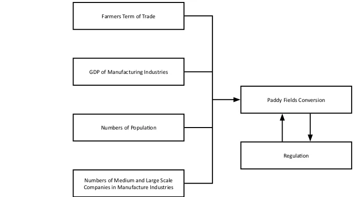
Farmers Term of Trade
GDP of Manufacturing Industries
Paddy Fields Conversion
Regulation Numbers of Population
Numbers of Medium and Large Scale Companies in Manufacture Industries
and paddy field conversion is negatively correlated with the farmers’ term of trade. Therefore, this study tries to determine the factors that influence the occurrence of paddy fields conversion based on
the farmers’ term of trade variable, an industrial development seen from the GDP of the industrial sector and the number of medium and large companies in the manufacturing industry and also the population variable.
To review it, this research is proposing three main questions. First, how is the growth of paddy field
conversion in Java? Second, what is the determinant
factors influencing paddy fields conversion in Java?
And third, how far is the regulations applied in order
to control paddy fields conversion.
Summarizing the above review, the framework
of this study can be illustrated as in Figure 1.
Research hypothesis can be described as
follows: first, presumed that paddy fields conversion
in Java is increasing. Second, the farmers’ term of trade, the GDP of manufacturing industries, numbers of the population, and numbers of medium and large scale companies in manufacturing industries
with significant influence towards paddy fields
conversion in Java.
This is based on previous research about the factors that affect paddy field conversion, one of
which is the research conducted by Kustiawan (1997)
which stated that the external factors that influence the occurrence of paddy fields conversion are the
regional development, population growth and GDP
growth. The greater the rate regional development,
the higher the rate of population growth and the greater the rate of GDP growth resulted in extensive
increases of paddy field conversion.
II. Method
The data used in this study is secondary data. The data consists of data on the size of paddy fields,
Gross Domestic Product (GDP) in manufacture
industries, farmers term of trade (NTP), numbers
of population, and numbers of medium and large scale companies in manufacturing industries in 5 provincial regions in Java, namely west Java, central Java, Yogyakarta, East Java, and Banten with time
period 1995-2013. The data is collected by learning, studying, and analyzing the source of literature in
the form of statistical data from the published data,
books, and scientific journals that are relevant to the
research.
The collected data then processed and analyzed in order to answer the problems in research. The
analytical method used is quantitative descriptive analysis and statistical analysis using multiple
linear regression methods to test the significance of
the variables through F test and partial correlation.
A. Quantitative Descriptive Analysis
The quantitative descriptive analysis is a method to describe paddy fields conversion that occurred on the island of Java. The analysis is
performed using a mathematical formula as follows:
(∁t-At)=Lt-Lt-1
Paddy fields conversion is defined as net paddy fields conversion. This means that paddy fields area in year t (Lt) is the paddy fields area of the previous year (Lt-1) plus the new paddy fields (Ct) and the reduced paddy fields (At). Thus, if the paddy fields conversion is positive, it means a new paddy field
occurs more comprehensive, respectively in year
t. Conversely, if the paddy fields conversion is negative, meaning that paddy fields reduced wider than new paddy fields, respectively in year t (Ilham
et al., 2005).
B. Statistical Analysis
In accordance with the objectives and hypothesis of the research, the relationship between
variables can be described specifically in multiple
linear regression models (Juanda & Junaidi, 2012).
This analysis can be used to describe the extent of
reliance is the dependent variable by one or more independent variables. Based on the variables that described the multiple linear regression models, it was formulated as follows:
Y=a+b1 X1it+b2 X2it+b3 X3it+b4 X4it+et
Information:
Y = The rate of paddy fields conversion
growth to provincial -i, the time period
-t (%)
X1 = The rate of farmers term of trade growth to provincial -i, the time period
-t (%)
X2 = The rate of GDP manufacturing industries growth to provincial -i, the time period -t (%)
X3 = The rate of population growth provincial -i, the time period -t (%) X4 = The rate of medium and large number
of companies in the manufacturing industry growth provincial -i, the time period -t (%)
a = Constanta
b1, b2, b3 = regression coefficient eit = error factors
The data used in the analysis is panel data
data regression model (Firdaus, 2011), namely:
(1) Common-Constant Method (The Pooled OLS
Method or PLS), (2) Fixed Effect Method (FEM), and (3) Random Effect method (REM). Furthermore, this
equation models are analyzed using the program
Eviews 7.0 for estimating the determinant factors of
paddy fields conversion on Java in 1995-2013.
III. Results and Discussion
A. The Growth of Paddy Fields Conversion in Java
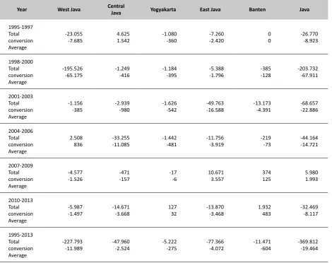
The growth of paddy fields conversion in this study is analyzed by looking at the changes in paddy fields area in each Java province. The growth of paddy fields conversion in Java in 1995-2013 can be seen in Table 1. Based on Table 1, it can be seen that during the year 1995-2013, paddy fields conversion
occurs in all provinces in Java with a total conversion of about 370 thousand hectares, or approximately
19 thousand hectares annually. This trend indicates that paddy fields conversion is greater than the new paddy fields. This conversion includes conversion of paddy field into non-agricultural activities such as
industrial or service industries and conversion to
agricultural activities other than paddy fields such
as farm or plantation and horticulture.
Based on Table 1, the highest paddy fields
conversion occurred during the year 1998-2000
with total paddy fields converted about 204
thousand hectares or approximately 68 thousand
hectares annually. This shows that in the period of economic crisis, paddy fields conversion increased
sharply compared to the previous period in which
the paddy fields conversion in 1995-1997, during this period paddy field converted about 27 thousand
hectares. Compared to the previous period, the
Table 1.
Growth of Paddy Fields Conversion by Province in Java of 1995-2013 (Ha)
Year West Java Central
Java Yogyakarta East Java Banten Java
1995-1997
paddy field conversion is increased about 7.6%. The
economic crisis led to unemployment rising and the subsequent cause a decrease in public revenue.
This situation triggered the paddy fields conversion.
Most people who only have assets in the form of
paddy fields will sell the land to maintain living to
those who earn high incomes.
Along with the increasing of economic level
post economic crisis, the paddy field conversion is
reduced, it can be seen throughout the year
2001-2003 which the amount of paddy field conversion
is 69 thousand hectares reduced about 44 thousand hectares from the year 2004-2006. In the period
2007-2009 the overall paddy fields conversion even
be positive, meaning that the number of new paddy
fields is higher than the reduced paddy fields. The new paddy field occurs about 6 thousand hectares.
However, unfortunately, this condition does not
last long, the paddy fields conversion in Java occurs
again in 2010-2013 and reduced about 32 thousand
hectares paddy field or about 8 thousand hectares annually. It indicates that the paddy field conversion
still cannot be controlled.
Based on paddy field conversion that occurs in all province in Java, paddy field conversion in West Java province is higher compared to other provinces. Throughout the Years 1995-2013 West Java Province experienced paddy field Conversion
about 228 thousand hectares or about 12 thousand
hectares per year. West Java province is also the
province which experienced the sharpest increase
of paddy field conversion on economic crisis
period that is about 195 thousand hectares or
increased about 8.5% from the size of paddy field
conversion in the previous years. East Java is in the second position which experienced higher paddy
fields conversion. During 1995-2013, paddy field
conversion at central Java is about 77 hectares.
That was followed by Central Java at 48 thousand hectares. Paddy field conversion in Banten Province is in the fourth position that the paddy field reduces
about 11,5 thousand hectares, and followed by DIY of about 5 thousand hectares.
The growth of paddy field conversion is also seen by a paddy field conversion rate. Paddy field
conversion rate indicates the percentage of paddy
field conversion speed that occurs in each province in Java. The rate of paddy field conversion by provinces in Java in 1995-2013 can be seen in Table
2.
Based on Table 2, it can be seen that the net rate of paddy fields conversion in Java over the period 1995 to 2013 is about 0.57% per year. West
Java Province experienced the highest rate of paddy
field conversion compared to other provinces in
Java, in which the value is about 1.07% per year.
The second position is experienced by Yogyakarta province with a paddy field conversion rate of about
0.47% per year. Third and fourth highest paddy field conversion rate in Java is occupied by East Java province with net paddy fields conversion rate of about 0.36% per year and Banten with paddy fields
conversion rate of about 0.29% per year, while the
last position with lowest paddy field conversion
Table 2.
Paddy Field Conversion Rate by Province in Java, the year of 1995-2013
Province
Paddy Field Conversion Rate at the average net per
year (%)
West Java 1.07
Central Java 0.26
Yogyakarta 0.47
East Java 0.36
Banten 0.29
Java 0.57
Source: Statistics Indonesia (BPS), 1995-2013 (processed)
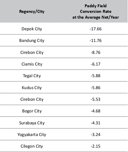
Table 3.
Paddy Field Conversion Rate by Regency/City in Java, Year 2009-2013
Regency/City
Paddy Field Conversion Rate at the Average Net/Year
Depok City -17.66
Bandung City -11.76
Cirebon City -8.76
Ciamis City -6.17
Tegal City -5.88
Kudus City -5.86
Cirebon City -5.53
Bogor City -4.68
Surabaya City -4.31
Yogyakarta City -3.24
Cilegon City -2.15
rate throughout the years 1995-2013 is occupied by Central Java province at 0.26% per year.
Based on the growth of paddy field conversion
in all cities/regencies in Java in the last 5 years
(2009-2013), it shows that in general, Paddy field
conversion rate is the highest in urban areas, as
shown in Table 3.
Based on Table 3, in the period of 2009-2013, the highest paddy field conversion rate is dominated
by Urban area. Depok city experienced the highest
paddy field conversion rate at 17.66%, followed
by Bandung city on the second position with
11.76%. third, fourth and fifth position, respectively
occupied by Cirebon regency (8.76%), Ciamis
regency (6.17%) and Tegal city (5.88%). Table 3
also shows that the region with the highest paddy
field conversion is dominated by areas in West Java
province, such as Depok city, Bandung city, Cirebon regency, Ciamis regency, Cirebon city and Bogor
city (4.68%). The region that experienced highest paddy field conversion rate in Central Java province is Tegal city and Kudus regency (5.86%). The region experienced highest paddy field conversion rate in East Java province is Surabaya city with paddy field
conversion rate in 4.31%. Yogyakarta is a region
which suffered the highest paddy field conversion Rate in Yogyakarta province is at 3.24%, While the highest paddy field conversion rate in Banten
province is occupied by the city of Cilegon by 2.15%.
B. Determinant Factors of Paddy Fields Conversion in Jawa
The determinant factors that influence paddy fields conversion in Java in this study were analyzed
based on the effect of the farmers’ term of trade, GDP of manufacturing industries sector, numbers of population and number of medium and large
companies in the manufacturing industries.
Determination of the independent variables is based on previous research, especially research conducted by Ilham et al (2005) about the
development and the factors that affect paddy fields
conversion in Indonesia, where the independent variable used in this study is also one of the variables used in the study. Farmers’ term of trade as a proxy for the competitiveness of agricultural products, especially rice; GDP of the industrial sector and the number of medium and large companies in the manufacturing industry as a proxy for industrial development, as well as a population as a proxy for residential needs.
These factors are calculated based on data
from BPS between 1995 and 2013 from 5 Provinces in Java by using Eviews 7.0.
3) Regression Analysis
The model equations are obtained based on
the results of the estimation Pool Ordinary Least Square (PLS) method, Fixed Effects Model (FEM) Method and Random Effects Model (REM) Method respectively as follows:
a) Pool Ordinary Least Square (PLS) Method
The model equations are obtained
based on the results of the estimation Pool Ordinary Least Square method (PLS) is as follows:
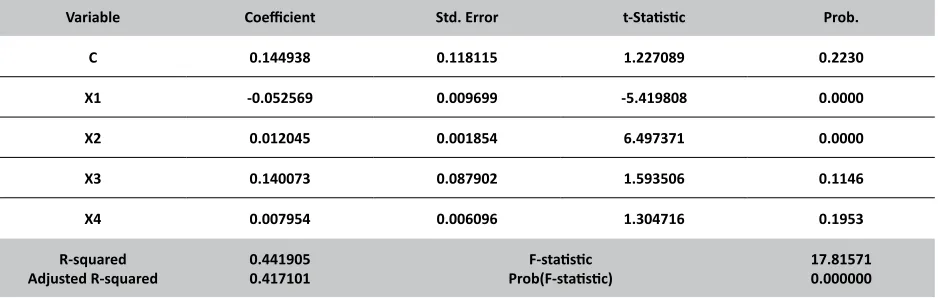
Y=0.145-0.0526X1+0.012X2+0.140X3+0.008X4
The estimation results using Pool
Ordinary Least Square (PLS) Method in
the form of value coefficients, standard
errors, t-statistics and analysis results are
Table 4.
The Estimation Results Using Pool Ordinary Least Square (PLS) Method
Variable Coefficient Std. Error t-Statistic Prob. C 0.144938 0.118115 1.227089 0.2230 X1 -0.052569 0.009699 -5.419808 0.0000 X2 0.012045 0.001854 6.497371 0.0000 X3 0.140073 0.087902 1.593506 0.1146 X4 0.007954 0.006096 1.304716 0.1953 R-squared
Adjusted R-squared
0.441905 0.417101
F-statistic
Prob(F-statistic) 17.815710.000000
presented in Table 4.
b) Fixed Effect Model (FEM) Method
The model equations are obtained
based on the results of the estimation using Fixed Effect Model (FEM) is as follows:
Y=0219+D-0.0543X1+0.0119X2+0.120X3+0.007X4
In equations using FEM method, the slope for farmers term of trade, the GDP of manufacturing industries sector, numbers of population and the number of medium and large companies in the processing industries applicable to all regions i, but
the intercept every region is different, depending on the value of the dummy
(Di). The coefficient of basic, standard
errors, t-statistics and analysis results are
presented in Table 5.
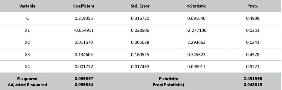
c) Random Effect Model (REM) Method
The model equations are obtained
based on the results of the estimation using Random Effect Model (REM) is as follows:
Y=0219-0.065X1+0.0117X2+0.135X3+0.002X4
In the equation using the method of this method, error component of each
Table 5.
The Estimation Results Using Fixed Effect Models (FEM) Method
Variable Coefficient Std. Error t-Statistic Prob. C 0.218752 0.141169 1.549577 0.1249 X1 -0.053836 0.009472 -5.683664 0.0000 X2 0.011915 0.001801 6.615373 0.0000 X3 0.119965 0.089746 1.336719 0.1848 X4 0.007233 0.006050 1.195664 0.2351
Cross-section fixed (dummy variables)
R-squared Adjusted R-squared
0.458628 0.408268
F-statistic
Prob(F-statistic) 9.1069710.000000
Source: Statistics Indonesia (BPS), 1995-2013 (processed)
Table 6.
The Estimation Results Using Random Effect Models (REM) Method
Variable Coefficient Std. Error t-Statistic Prob.
C 0.219056 0.316720 0.691640 0.4909
X1 -0.064911 0.028506 -2.277106 0.0251
X2 0.011670 0.005088 2.293663 0.0241
X3 0.134603 0.180525 0.745623 0.4578
X4 0.001712 0.017463 0.098011 0.9221
R-squared Adjusted R-squared
0.099697 0.059684
F-statistic
Prob(F-statistic) 2.4915960.048615
region is different. The coefficient of
basic, standard errors and t-statistics and
analysis results are presented in Table 6.
Based on several methods above, then some tests are used to choose which method is the most
appropriate. Chow Test or Likelihood Ratio Test is
used to chose which one is more appropriate for
PLS and FEM methods. The estimation results of Chow Test or Likelihood Ratio Test using Eviews 7.0 can be seen in Table 7. The test results showed that
the probability for the Cross-section F is 0,9211, which is over 0.05 (Decision: accept Ho), Ho, in this case, indicates that the PLS method is better than FEM method, so it can be concluded that in 95%
confidence level, PLS method is better than the FEM
method.
Hausman test is used to find the appropriate
method between FEM and REM method. Based on
the result of Hausman test in Table 8, it shows that
the probability value for the Cross-section F is over 0.05, which indicates the condition accepts Ho.
In this case, Ho is indicating the REM is better than FEM method. So that as the value of probability for the Cross-section F is 0,7055, it can be concluded
that in 95% confidence level, REM method is better
than FEM method.
Based on the result of a series of estimates above, it can be seen that the model equations generated by the PLS method is better in explaining
the influence of variable farmers’ term of trade,
number of population and the number of medium and large companies in the manufacturing
industries of the vast paddy fields research areas.
Based on estimates by PLS method, obtained the following equation:
Y=0.145-0.053X1+0.012X2+0.140X3+0.008X4
The equation shows that:
1. C constant value of 0.145 means that if the farmers’ term of trade, the number of population, and the number of medium and large companies in the manufacturing
industries is 0, then the paddy fields conversion
will grow to 0.145%.
2. b(X1) = -0.053 means that if the farmers’ term of trade is increased by 1%, while other variables
remained, then the paddy fields conversion (Y)
will be decreased by 0.053%. Sign (-) indicates a negative correlation between the inverse or opposite of the farmers’ term of trade and
paddy fields conversion, that is, if the farmers’ term of trade is high, then the paddy field
conversion will be low.
3. b(X2) = 0.012 means that if the variable GDP of manufacturing industries sector increased by 1%, while other variables remained, the
paddy fields conversion (Y) will be increased
by 0.012%. Sign (+) positive indicates the same direction of the relationship between the GDP of manufacturing industries sector and
conversion of paddy fields, that is, if the GDP
of manufacturing industries sector is high then
the paddy field conversion will also be high.
4. b(X3) = 0.140 means that if a variable number of population increased by 1%, while other
variables remained, the paddy fields conversion
(Y) will increase by 0.140%. Sign (+) positive indicates the same direction relationship between the number of population and the
paddy fields conversion that is, if the number of population is high, the paddy fields conversion
will also be high.
Table 7.
The Estimation Result of Likelihood Test Ratio Between FEM and PLS Method
Effects Test Statistic d.f. Prob.
Cross-section F 0.229591 (4.86) 0.9211
Source: Statistics Indonesia (BPS), 1995-2013 (processed)
Table 8.
The Estimation Result of Hausman Test Between FEM and REM Method
Test Summary Chi-Sq. Statistic Chi-Sq. d.f. Prob.
Cross-section random 2.164429 4 0.7055
5. b(X4) = 0.008 means that if a variable number of medium and large companies in the manufacturing industry is increased by 1%,
while other variables remained, the paddy fields
conversion (Y) will be increased by 0.008%. sign (+) positive indicates the same direction relationship between the number of medium and large companies in the manufacturing
industries and paddy fields conversion, that is,
if the number of medium and large companies in the manufacturing industries is high then
paddy fields conversion is also high.
4) Classical Assumption Test
To be accepted as a multiple linear regression
model assumption, it must meet the Classic assumption test, which includes:
a) Normality Test
Based on the test results of normality treated with 7.0 eviews program, it can be obtained that the shape of the histogram is distributed asymmetrically so that we expected residuals to be normally distributed. Based on statistical test Jargue bera statistical value of 1.528706 with 46.56% probability, it can be concluded that the residuals were normally distributed and pass the test for normality so that testing data is appropriate to proceed in the study.
b) Multicollinearity Test
From the data processing through the eviews 7.0 program, it can be concluded: • The correlation coefficient for the
variable farmer term of trade and the GDP of manufacturing industries sector amounted to -0.210224.
This means that Multicollinearity
does not happen between variable rate and the GDP manufacturing industries because of the correlation
coefficient is less than 0.8. Then we
can say “pass the Multicollinearity test “.
• The correlation coefficient for the variable of farmers’ term of trade and the number of
population at 0.121284. This means
Multicollinearity does not happen between the term of trade variable and a population of farmers because the magnitude of the correlation
coefficient is 0.121284 less than
0.8, it can be said to “pass the Multicollinearity test “.
• The correlation coefficient for the
variable farmer’s term of trade and the number of medium and large companies in the manufacturing industries of -0.016026. this means not happen Multicollinearity between the farmer’s term of trade variable and number of medium and large companies in the manufacturing industries because the magnitude of the correlation
coefficient is -0.016026 less than
0.8 then we can say “pass the Multicollinearity test “.
• The correlation coefficients for variables GDP of manufacturing industries sector and a number of the population are -0.548850. this means not happen Multicollinearity between GDP of manufacturing industries sector variables and a number of population. because the magnitude of the correlation
coefficient is -0.548850 less than
0.8, then we can say “pass the Multicollinearity test “.
• The correlation coefficients for GDP of manufacturing industries sector variables and the number of medium and large companies in the manufacturing industries are -0.005481. this means Multicollinearity does not happen between GDP of manufacturing industries sector variable and a number of medium and large companies in the manufacturing industries because of the magnitude
of the correlation coefficient is
-0.005481 less than 0.8 then we can say “pass the Multicollinearity test “. • The correlation coefficients for the
number of population variables and the number of medium and large companies in the manufacturing industries are -0.045813. this means not happen Multicollinearity between a number of population variables and the number of medium and large companies in the manufacturing industries because the magnitude of the correlation
coefficient is l-0.045813 ess than
0.8 then we can say “pass the Multicollinearity test “.
c) Heteroskedasticity Test
Based on heteroscedasticity test
that the probability value Obs * R-squared are 0.2769. Because the probability value Obs * R-squared are 0.2769 > 0.05, there is no heteroscedasticity.
d) Test Autocorrelation
Based on Autocorrelation test
through eviews 7.0 program, we can find
that the probability value Obs * R-squared are 0.5006. Because the probability value Obs * R-squared are 0.5006 > 0.05 can be concluded that in this research model passes autocorrelation test.
e) Test of linearity
Based on the linearity test through eviews 7.0 program, we know the value
of the F probability of 0.6352. Thus, the
probability of 0.6352 > 0.05 so that we can conclude this research model linearity test passes.
5) Hypothesis Testing
a) t-Test
• Farmers’ term of trade variable Based on the estimation by eviews 7.0 program for farmers’ term of trade variable, the result obtained
probability value (significance) = 0.0000. Thus because of the probability value less than α 0.05
(0.0000 < 0.05). It can be concluded that the farmers’ term of trade
variable significantly influences the paddy fields conversion in Java.
• The GDP of manufacturing industries sector Variable
Based on the estimation by eviews
7.0 program for The GDP of
manufacturing industries sector Variable, the result obtained
probability value (significance) = 0.0000. Thus because of the probability value is less than α 0.05
(0.0000 < 0.05), it can be concluded that the GDP manufacturing
industries variables significantly influence the paddy fields conversion
in Java.
• The numbers of population Variable Based on the estimation by eviews 7.0 program for the number of population variable, the result obtained probability value
(significance) = 0.1146. Thus
because of the probability value less
than 0.05 α (0.1146 < 0.05), it can be
concluded that a variable number of
the population did not significantly influence paddy fields conversion in
Java.
• The number of medium and large companies in the manufacturing industries Variable
Based on the estimation by eviews 7.0 program for a number of medium and large companies in the manufacturing industries Variable, the result obtained the probability
value (significance) = 0.1953. Thus
because of the probability value is
less than 0.05 α (0.1953 < 0.05), it
can be concluded that the number of medium and large companies in the manufacturing industries Variable
did not significantly influence paddy fields conversion in Java.
b) F Test
Based on the estimation by eviews 7.0 program, probability value obtained for the F-statistic is equal to 0.000000.
Thus because of the probability value (significance) is greater than α 0.05
(0.000000 > 0.05). It can be concluded that simultaneously, the farmers’ term of trade, the GDP of manufacturing industries sector, the number of population, and the number of medium and large companies in the manufacturing industries variables
significantly influence the paddy fields
conversion in Java.
6) Coefficient of Determination
Based on the estimation through the program
eviews 7.0, the coefficient of determination can be seen from the adjusted R-Squared value. The
result for adjusted R-Squared value is 0.417101.
This means that 41.71% of paddy fields conversion in Java is influenced by farmers’ term of trade, the
number of population and the number of medium and large companies in the manufacturing industries
variables, while the remaining 58.29% is influenced
by other variables which are not examined in this study.
Based on the results of the analysis determined by using the PLS (Pool Ordinary Least Square) method, it can be seen that together (simultaneously) the farmers’ term of trade, the GDP of manufacturing industries sector, the number of population, and the number of medium and large companies in the manufacturing industries variables
significantly influence paddy fields conversion in
of 0.417101 indicates that 41.41% of paddy fields conversion in Java is influenced by farmers’ term of
trade, the number of population, and the number of medium and large companies in the manufacturing industries variables, while the remaining 58.29% is
influenced by other variables not examined in this
study.
Based on the research, we find that the farmers’ term of trade significantly influence the paddy field conversion in Java is in accordance with the initial hypothesis of the study. The low term of
trade caused no incentive for farmers to continue to
live in their paddy field production, so they tend to convert their paddy fields (Ashari, 2003). Similarly,
the GDP of manufacturing industries sector variable
significantly influenced paddy fields conversion, it indicates that industrial activities and the size of the
role of the industrial sector in the GDP stimulated government priorities to shift from agriculture to the industrial sector. For farmers, the increase in industrial sector becomes one of the factors to switch professions to become workers in the industrial sector and convert their land into other
uses rather than the paddy field.
Based on the estimation by eviews 7.0 program for the number of population variable, the result
obtained probability value (significance) = 0.1146. Thus because of the probability value is less than 0.05 α (0.1146 < 0.05), the number of population variable did not significantly influence paddy field
conversion. Based on the estimation by eviews 7.0 program for the medium and large companies in the manufacturing industry variable, the result
obtained probability value (significance) = 0.1953. Thus, because the probability value is less than 0.05 α (0.1953 < 0.05), It can be concluded that
the number of medium and large companies in the manufacturing industries variable did not
significantly influence paddy fields conversion in Java. This result shows that both variables did not
correspond to the initial hypothesis of the studies.
The negative slope of the variables equation
such as on farmers’ term of trade variable pointed out that the increase of farmers’ term of trade will
cause the decrease of the paddy field conversion. In
contrast, the positive slope such as on the GDP of manufacturing industries sector pointed out that the increase in GDP of manufacturing industries sector
caused the increase in paddy field conversions.
One of the interesting properties in empirical
research model is that the slope coefficient (β)
measure the elasticity of Y with respect to X, or in other words, the percentage change in Y for a given percentage change in X (Gujarati, 2007). In
symbolic, if ΔY indicated the changes of paddy field conversion (Y) and ΔX indicated the changes in a variable that influence paddy field conversion (X), then it can be defined as a coefficient of elasticity
(E). Elasticity criteria are as follows:
• E > 1 = elastic • E < 1 = inelastic • E = 1 = uniter
• E = 0 = perfectly inelastic • E = ~ = perfectly elastic
As for the influence of these variables, it can be
seen in the estimated equation below:
Y=0.145-0.053X1+0.012X2+0.140X3+0.008X4
From the equation, we can conclude the elasticity of each variable. Based on a slope, the value of Farmers’ term of trade variable amounted to -0.053, it can be seen that the elasticity value of Farmers’ term of trade variable towards paddy
fields conversion is -0.053. Based on a slope, the
value of GDP of manufacturing industries sector variable amounts to 0.012, it can be seen that the elasticity value of GDP of manufacturing industries
sector variable towards paddy fields conversion is
0.012.
Based on elasticity value of the farmers’ term of trade variable and the GDP of manufacturing industries sector variable which is smaller than 1, it is indicated that the farmer’s term of trade variable and the GDP of manufacturing industries
sector variable are inelastic towards paddy fields
conversion. It showed that every 1% increase in the
farmers’ term of trade will decrease paddy fields
conversion amounted to 0.053%. Instead, each 1% increase in the GDP of manufacturing industries
sector will improve paddy fields conversion
amounted to 0.012%.
C. Government Regulations to Control Paddy Fields Conversion
Paddy field is a private good that is legal to be transacted. Therefore, the efforts to limit the occurrence of paddy field conversion can be done is merely control. The control should be the start
from the factors that cause the occurrence of paddy
fields conversion, there are economic, social, and
legal instruments (Ilham et al., 2005). One of the efforts made by the government to control the
conversion of paddy fields is through a juridical
government regulation.
However, the actual fact showed that the
control of paddy fields conversion through juridical approach is not maximized in overcoming problems of paddy fields conversion. Lichtenberg & Ding
(2008) states that the biggest obstacle in the protection of agricultural land is institutional aspect rather than on the physical aspects. Failure to set the institutional aspects affect the demand and supply of land to be converted. A juridical instrument that has been developed by the government have not applied clear sanctions, overlapping and not supported by economic and social instruments (Irawan, 2008).
This causes the paddy fields conversion rate is still quite large even venturing into paddy fields with
technical irrigation potential for rice production. For example, the implementation of Law of the Republic of Indonesia Number 41 of 2009 is plagued with the overlapping rules of other laws, such as Law of the Republic of Indonesia Number 23 of 2014 on Regional Government, where the Regional Government has authority to assign a function area. Agriculture is only a matter of choice for Regency/City Government in the Law of the Republic of Indonesia Number 23 of 2014.
These conditions increase the chances of ignoring
local agricultural sector. Irawan (2008) states that regional Government focus on the progress of their region that viewed from the economic growth and
revenue (PAD), The Regional Government are trying
to increase investment in the non-agricultural sector as it can generate greater revenue and promote faster economic growth. Consequently, if the case demands conversion of agricultural land to be used for other nonagricultural uses, the local government is less likely to consider a ban on land conversion applicable.
Furthermore, inconsistency between
paddy fields conversion control objectives and determining the extent of paddy fields in the spatial
instrument can also trigger the occurrence of paddy
fields conversion. This can be seen in the research
conducted by Dewi (2010) which showed that
the Spatial Plan/RTRW as an instrument layout is precisely triggered by the occurrence of paddy fields conversion. This occurs due to the incompatibility of determining the extent of paddy fields contained in the RTRW with the actual area where it turns paddy fields area listed in the RTRW are smaller than the actual paddy fields. For example, The Study which comparing two RTRW in Bekasi Regency year 1999 and 2007 showed that in the RTRW 1999, vast areas allocated for paddy fields is 66.937 hectares, while in RTRW 2007, the area designed for paddy fields decreased into 51.093 Ha. This means that there has been a decline in the paddy fields area. In addition,
through spatial analysis, it is known that based on
the facts, the actual paddy fields area is larger than
stated in RTRW 2007, which is consist of the area for technical irrigated paddy fields amounted to 58.680 Ha and rainfed paddy fields area amounted to 2.486 Ha. This means that there is an actual technical irrigated paddy field amounted to 18.400 Ha that is not included in the allocation of paddy fields designation on RTRW 2007 so that it can stimulate the occurrence of paddy fields conversion in those areas. Thus, based on the case above, it turns
the spatial instrument that expected to provide
protection for paddy fields precisely triggering the occurrence of greater paddy fields conversion.
IV. Conclusion
Based on the estimation result it can be
seen that during the year 1995-2013 paddy field
conversion occurs at all provinces in Java with total conversion about 370.000 Ha, or about 19.000 Ha/ year, with conversion rate are about 0.57% annually.
West Java Province experienced the largest paddy field conversion in Java throughout the years
1995-2013 with total conversion about 228.000 Ha, or about 12.000 Ha/year.
Based on the resulting equation models, can be seen that the farmers’ term of trade variable and
GDP of manufacturing industries sector significantly influences the paddy fields conversion in Java. Based
on the slope and the elasticity, in partial, it is known that each 1% increase in the farmers’ term of trade
will be lowered paddy fields conversion amounted
to 0.069%. Instead, each 1% increase in the GDP of the manufacturing industries will improve paddy
field conversion amounted to 0.287%, where the
slope value of less than 1 indicates that the farmers’ term of trade variable and GDP of manufacturing
industries sector are inelastic towards paddy fields
conversion.
Moreover, paddy fields conversion in Java needs
to be controlled considering the vast reduction of
paddy fields area in Java. Efforts to control paddy fields conversion in Java can be done by reducing the factors that affect paddy fields conversion. The effort required in order to reduce the paddy fields conversion in Java is to fix the farmers term of trade, especially paddy fields farmers and do monitoring
in industries developments in order not to convert a
paddy fields for the industrial expansion, that is the
policy of increasing the purchasing power of farmers so that farmers term of trade increased. Besides that, it also needs policies in land conversion control due to the development of industrial activities such as monitoring the granting of land use, especially
paddy fields for other uses.
However, currently, the regulations to protect agricultural land still have not effective enough to
overcome problems of paddy fields conversion into
and have not applied clear sanctions, and also
inconsistency between paddy fields conversion
control objectives and determining the extent of
paddy fields in the spatial instrument still being obstacle in order to control paddy fields conversion
in Java and in fact, precisely trigger the occurrence
of greater paddy fields conversion.
Acknowledgement
First of all, praise to Allah, SWT for his mercy
and guidance in giving me full strength to complete this Paper. A lot of thanks to my tutors Prof. Dr. Ir.
DS Priyarsono and Prof. Dr. Ir. Noer Azam Achsani
from Bogor Agricultural University (IPB), for their support, research assistant and valuable comments to revise the Paper. Great appreciation to the Research and Development Centre of Ministry of Agrarian and Spatial Planning for giving me permission and supports during conducting the paper. Also Special thanks to my families for the extraordinary supports.
V. References
Azadi, H., Ho, P., & Hasfiati, L. (2010). Agricultural
land conversion drivers: A comparison between less developed, developing and developed countries. Land Degradation & Development, 22(6), 596–604. http://doi.org/10.1002/ ldr.1037
Butar-Butar, E. G. V. (2012). Analisis
Faktor-faktor Konversi Lahan Sawah Irigasi Teknis
di Provinsi Jawa Barat. Bogor Agricultural University. Retrieved from http://repository. ipb.ac.id/handle/123456789/56144
Dewi, I. A. (2010). Analisis Efektifitas Tata Ruang
sebagai Instrumen Pengendali Perubahan Penggunaan Lahan Sawah menjadi Penggunaan Lahan Non Pertanian di Kabupaten Bekasi. School of Business - Bogor Agricultural University.
Firdaus, M. (2011). Aplikasi Ekonometrika untuk
Data Panel dan Time Series. Bogor: IPB Press.
Hidayat, S. I. (2008). Analisis Konversi Lahan Sawah
di Propinsi Jawa Timur. J-SEP, 2(3), 48–58.
Retrieved from http://jurnal.unej.ac.id/index. php/JSEP/article/view/431
Ilham, N., Syaukat, Y., & Friyatno, S. (2005). Perkembangan dan Faktor-faktor yang Mempengaruhi Konversi Lahan Sawah serta Dampak Ekonominya. SOCA (Socio-Economic of Agriculture and Agribusiness), 5(2), 1–25. Retrieved from http://ojs.unud.ac.id/index. php/soca/article/view/4081
Irawan, B. (2008). Meningkatkan Efektifitas
Kebijakan Konversi Lahan. FORUM
PENELITIAN AGRO EKONOMI, 26(2), 116–131.
Retrieved from http://pse.litbang.pertanian. go.id/ind/index.php/publikasi/forum-agro-
ekonomi/312-forum-agro-ekonomi-vol26-
no02-2008/2084-meningkatkan-efektifitas-kebijakan-konversi-lahan
Irawan, B., Purwoto, A., Dabukke, F. B. M., &
Trijono, D. (2012). Studi Kebijakan Akselerasi
Pertumbuhan Produksi Padi di Luar Pulau Jawa. Retrieved from http://pse.litbang. pertanian.go.id/ind/index.php/laporanh a s i l p e n e l i t i a n / 2 5 3 0 l a p o r a n pertanian.go.id/ind/index.php/laporanh a s i l -penelitian-2012
Isa, I. (2006). Strategi Pengendalian Alih Fungsi Lahan Pertanian. In A. Dariah, N. L. Nurida, Irawan, E. Husen, & F. Agus (Eds.), Prosiding Seminar Multifungsi dan Revitalisasi Pertanian (pp. 1–16). Jakarta: Indonesian Agency for Agricultural Research & Development, Ministry of Agriculture; Ministry of Agriculture, Forestry and Fisheries, Japan; ASEAN Secretariat. Retrieved from http://balittanah.litbang. pertanian.go.id/ind/index.php/en/publikasi-mainmenu-78/27-prosiding3
Isa, I. (2014). Alih Fungsi Lahan dan Ketahanan
Pangan: Konflik Penggunaan Tanah. Jakarta.
Juanda, B., & Junaidi. (2012). Ekonometrika Deret
Waktu : Teori dan Aplikasi. Bogor: IPB Press.
Law of the Republic of Indonesia Number 12 of 1992 concerning Plant Cultivation System, Pub. L. No. 12 (1992). Indonesia.
Law of the Republic of Indonesia Number 26 of 2007 on Spatial Planning, Pub. L. No. 26 (2007). Indonesia.
Law of the Republic of Indonesia Number 41 of 2009 on Sustainable Land Farming Protection, Pub. L. No. 41 (2009). Indonesia.
Law of the Republic of Indonesia Number 5 of 1960 on the Basic Regulation of Agrarian Principles, Pub. L. No. 5 (1960). Indonesia.
Lichtenberg, E., & Ding, C. (2008). Assessing farmland protection policy in China. Land Use Policy, 25(1), 59–68. http://doi.org/10.1016/j. landusepol.2006.01.005
Suriyanto, A. (2012). Analisis Beberapa Variabel yang Mempengaruhi Konversi Lahan Pertanian di Kabupaten Sidoarjo. Universitas Negeri Surabaya.
TB, C., Purwanto, J., F, R. U., & Ani, S. W. (2010).
Dampak Alih Fungsi Lahan Pertanian ke Sektor
Non Pertanian Terhadap Ketersediaan Beras di Kabupaten Klaten Provinsi Jawa Tengah. Caraka Tani, XXV(1), 38–42. Retrieved from