A.K. JAIN
Michigan State University
M.N. MURTY
Indian Institute of Science
AND
P.J. FLYNN
The Ohio State University
Clustering is the unsupervised classification of patterns (observations, data items, or feature vectors) into groups (clusters). The clustering problem has been
addressed in many contexts and by researchers in many disciplines; this reflects its broad appeal and usefulness as one of the steps in exploratory data analysis. However, clustering is a difficult problem combinatorially, and differences in assumptions and contexts in different communities has made the transfer of useful generic concepts and methodologies slow to occur. This paper presents an overview of pattern clustering methods from a statistical pattern recognition perspective, with a goal of providing useful advice and references to fundamental concepts accessible to the broad community of clustering practitioners. We present a taxonomy of clustering techniques, and identify cross-cutting themes and recent advances. We also describe some important applications of clustering algorithms such as image segmentation, object recognition, and information retrieval.
Categories and Subject Descriptors: I.5.1 [Pattern Recognition]: Models; I.5.3 [Pattern Recognition]: Clustering; I.5.4 [Pattern Recognition]: Applications— Computer vision; H.3.3 [Information Storage and Retrieval]: Information Search and Retrieval—Clustering; I.2.6 [Artificial Intelligence]:
Learning—Knowledge acquisition
General Terms: Algorithms
Additional Key Words and Phrases: Cluster analysis, clustering applications, exploratory data analysis, incremental clustering, similarity indices, unsupervised learning
Section 6.1 is based on the chapter “Image Segmentation Using Clustering” by A.K. Jain and P.J. Flynn,Advances in Image Understanding: A Festschrift for Azriel Rosenfeld(K. Bowyer and N. Ahuja, Eds.), 1996 IEEE Computer Society Press, and is used by permission of the IEEE Computer Society. Authors’ addresses: A. Jain, Department of Computer Science, Michigan State University, A714 Wells Hall, East Lansing, MI 48824; M. Murty, Department of Computer Science and Automation, Indian Institute of Science, Bangalore, 560 012, India; P. Flynn, Department of Electrical Engineering, The Ohio State University, Columbus, OH 43210.
Permission to make digital / hard copy of part or all of this work for personal or classroom use is granted without fee provided that the copies are not made or distributed for profit or commercial advantage, the copyright notice, the title of the publication, and its date appear, and notice is given that copying is by permission of the ACM, Inc. To copy otherwise, to republish, to post on servers, or to redistribute to lists, requires prior specific permission and / or a fee.
1. INTRODUCTION 1.1 Motivation
Data analysis underlies many comput-ing applications, either in a design phase or as part of their on-line opera-tions. Data analysis procedures can be dichotomized as either exploratory or confirmatory, based on the availability of appropriate models for the data source, but a key element in both types of procedures (whether for hypothesis formation or decision-making) is the grouping, or classification of measure-ments based on either (i) goodness-of-fit to a postulated model, or (ii) natural groupings (clustering) revealed through analysis. Cluster analysis is the organi-zation of a collection of patterns (usual-ly represented as a vector of measure-ments, or a point in a multidimensional space) into clusters based on similarity.
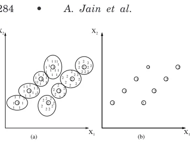
Intuitively, patterns within a valid clus-ter are more similar to each other than they are to a pattern belonging to a different cluster. An example of cluster-ing is depicted in Figure 1. The input patterns are shown in Figure 1(a), and the desired clusters are shown in Figure 1(b). Here, points belonging to the same cluster are given the same label. The variety of techniques for representing data, measuring proximity (similarity) between data elements, and grouping data elements has produced a rich and often confusing assortment of clustering methods.
It is important to understand the dif-ference between clustering (unsuper-vised classification) and discriminant analysis (supervised classification). In supervised classification, we are pro-vided with a collection of labeled (pre-classified) patterns; the problem is to label a newly encountered, yet unbeled, pattern. Typically, the given la-beled (training) patterns are used to learn the descriptions of classes which in turn are used to label a new pattern. In the case of clustering, the problem is to group a given collection of unlabeled patterns into meaningful clusters. In a sense, labels are associated with clus-ters also, but these category labels are data driven; that is, they are obtained solely from the data.
Clustering is useful in several explor-atory pattern-analysis, grouping, deci-sion-making, and machine-learning sit-uations, including data mining, document retrieval, image segmenta-tion, and pattern classification. How-ever, in many such problems, there is little prior information (e.g., statistical models) available about the data, and the decision-maker must make as few assumptions about the data as possible. It is under these restrictions that clus-tering methodology is particularly ap-propriate for the exploration of interre-lationships among the data points to make an assessment (perhaps prelimi-nary) of their structure.
The term “clustering” is used in sev-eral research communities to describe
CONTENTS
1. Introduction 1.1 Motivation
1.2 Components of a Clustering Task
1.3 The User’s Dilemma and the Role of Expertise 1.4 History
1.5 Outline
2. Definitions and Notation
3. Pattern Representation, Feature Selection and Extraction
4. Similarity Measures 5. Clustering Techniques
5.1 Hierarchical Clustering Algorithms 5.2 Partitional Algorithms
5.3 Mixture-Resolving and Mode-Seeking Algorithms
5.4 Nearest Neighbor Clustering 5.5 Fuzzy Clustering
5.6 Representation of Clusters
5.7 Artificial Neural Networks for Clustering 5.8 Evolutionary Approaches for Clustering 5.9 Search-Based Approaches
5.10 A Comparison of Techniques 5.11 Incorporating Domain Constraints in
Clustering
5.12 Clustering Large Data Sets 6. Applications
6.1 Image Segmentation Using Clustering 6.2 Object and Character Recognition 6.3 Information Retrieval
methods for grouping of unlabeled data. These communities have different ter-minologies and assumptions for the components of the clustering process and the contexts in which clustering is used. Thus, we face a dilemma regard-ing the scope of this survey. The produc-tion of a truly comprehensive survey would be a monumental task given the sheer mass of literature in this area. The accessibility of the survey might also be questionable given the need to reconcile very different vocabularies and assumptions regarding clustering in the various communities.
The goal of this paper is to survey the core concepts and techniques in the large subset of cluster analysis with its roots in statistics and decision theory. Where appropriate, references will be made to key concepts and techniques arising from clustering methodology in the machine-learning and other commu-nities.
The audience for this paper includes practitioners in the pattern recognition and image analysis communities (who should view it as a summarization of current practice), practitioners in the machine-learning communities (who should view it as a snapshot of a closely related field with a rich history of well-understood techniques), and the broader audience of scientific
profes-sionals (who should view it as an acces-sible introduction to a mature field that is making important contributions to computing application areas).
1.2 Components of a Clustering Task Typical pattern clustering activity in-volves the following steps [Jain and Dubes 1988]:
(1) pattern representation (optionally including feature extraction and/or selection),
(2) definition of a pattern proximity measure appropriate to the data do-main,
(3) clustering or grouping,
(4) data abstraction (if needed), and
(5) assessment of output (if needed).
Figure 2 depicts a typical sequencing of the first three of these steps, including a feedback path where the grouping process output could affect subsequent feature extraction and similarity com-putations.
Pattern representation refers to the number of classes, the number of avail-able patterns, and the number, type, and scale of the features available to the clustering algorithm. Some of this infor-mation may not be controllable by the
X X
practitioner. Feature selection is the process of identifying the most effective subset of the original features to use in clustering.Feature extraction is the use of one or more transformations of the input features to produce new salient features. Either or both of these tech-niques can be used to obtain an appro-priate set of features to use in cluster-ing.
Pattern proximityis usually measured by a distance function defined on pairs of patterns. A variety of distance mea-sures are in use in the various commu-nities [Anderberg 1973; Jain and Dubes 1988; Diday and Simon 1976]. A simple distance measure like Euclidean tance can often be used to reflect dis-similarity between two patterns, whereas other similarity measures can be used to characterize the conceptual similarity between patterns [Michalski and Stepp 1983]. Distance measures are discussed in Section 4.
The grouping step can be performed in a number of ways. The output clus-tering (or clusclus-terings) can be hard (a partition of the data into groups) or fuzzy (where each pattern has a vari-able degree of membership in each of the output clusters). Hierarchical clus-tering algorithms produce a nested se-ries of partitions based on a criterion for merging or splitting clusters based on similarity. Partitional clustering algo-rithms identify the partition that opti-mizes (usually locally) a clustering cri-terion. Additional techniques for the grouping operation include probabilistic [Brailovski 1991] and graph-theoretic [Zahn 1971] clustering methods. The variety of techniques for cluster forma-tion is described in Secforma-tion 5.
Data abstraction is the process of ex-tracting a simple and compact represen-tation of a data set. Here, simplicity is either from the perspective of automatic analysis (so that a machine can perform further processing efficiently) or it is human-oriented (so that the representa-tion obtained is easy to comprehend and intuitively appealing). In the clustering context, a typical data abstraction is a compact description of each cluster, usually in terms of cluster prototypes or representative patterns such as the cen-troid [Diday and Simon 1976].
How is the output of a clustering algo-rithm evaluated? What characterizes a ‘good’ clustering result and a ‘poor’ one? All clustering algorithms will, when presented with data, produce clusters — regardless of whether the data contain clusters or not. If the data does contain clusters, some clustering algorithms may obtain ‘better’ clusters than others. The assessment of a clustering proce-dure’s output, then, has several facets. One is actually an assessment of the data domain rather than the clustering algorithm itself— data which do not contain clusters should not be processed by a clustering algorithm. The study of cluster tendency, wherein the input data are examined to see if there is any merit to a cluster analysis prior to one being performed, is a relatively inactive re-search area, and will not be considered further in this survey. The interested reader is referred to Dubes [1987] and Cheng [1995] for information.
Cluster validity analysis, by contrast, is the assessment of a clustering proce-dure’s output. Often this analysis uses a specific criterion of optimality; however, these criteria are usually arrived at
Feature Selection/ Extraction
Pattern
Grouping Clusters Interpattern
Similarity Representations
Patterns
subjectively. Hence, little in the way of ‘gold standards’ exist in clustering ex-cept in well-prescribed subdomains. Va-lidity assessments are objective [Dubes 1993] and are performed to determine whether the output is meaningful. A clustering structure is valid if it cannot reasonably have occurred by chance or as an artifact of a clustering algorithm. When statistical approaches to cluster-ing are used, validation is accomplished by carefully applying statistical meth-ods and testing hypotheses. There are three types of validation studies. An external assessment of validity com-pares the recovered structure to an a priori structure. An internal examina-tion of validity tries to determine if the structure is intrinsically appropriate for the data. A relative test compares two structures and measures their relative merit. Indices used for this comparison are discussed in detail in Jain and Dubes [1988] and Dubes [1993], and are not discussed further in this paper.
1.3 The User’s Dilemma and the Role of Expertise
The availability of such a vast collection of clustering algorithms in the litera-ture can easily confound a user attempt-ing to select an algorithm suitable for the problem at hand. In Dubes and Jain [1976], a set of admissibility criteria defined by Fisher and Van Ness [1971] are used to compare clustering algo-rithms. These admissibility criteria are based on: (1) the manner in which clus-ters are formed, (2) the structure of the data, and (3) sensitivity of the cluster-ing technique to changes that do not affect the structure of the data. How-ever, there is no critical analysis of clus-tering algorithms dealing with the im-portant questions such as
—How should the data be normalized?
—Which similarity measure is appropri-ate to use in a given situation?
—How should domain knowledge be uti-lized in a particular clustering prob-lem?
—How can a vary large data set (say, a million patterns) be clustered effi-ciently?
These issues have motivated this sur-vey, and its aim is to provide a perspec-tive on the state of the art in clustering methodology and algorithms. With such a perspective, an informed practitioner should be able to confidently assess the tradeoffs of different techniques, and ultimately make a competent decision on a technique or suite of techniques to employ in a particular application.
There is no clustering technique that is universally applicable in uncovering the variety of structures present in mul-tidimensional data sets. For example, consider the two-dimensional data set shown in Figure 1(a). Not all clustering techniques can uncover all the clusters present here with equal facility, because clustering algorithms often contain im-plicit assumptions about cluster shape or multiple-cluster configurations based on the similarity measures and group-ing criteria used.
Humans perform competitively with automatic clustering procedures in two dimensions, but most real problems in-volve clustering in higher dimensions. It is difficult for humans to obtain an intu-itive interpretation of data embedded in a high-dimensional space. In addition, data hardly follow the “ideal” structures (e.g., hyperspherical, linear) shown in Figure 1. This explains the large num-ber of clustering algorithms which con-tinue to appear in the literature; each new clustering algorithm performs slightly better than the existing ones on a specific distribution of patterns.
informa-tion can also be used to improve the quality of feature extraction, similarity computation, grouping, and cluster rep-resentation [Murty and Jain 1995].
Appropriate constraints on the data source can be incorporated into a clus-tering procedure. One example of this is mixture resolving [Titterington et al. 1985], wherein it is assumed that the data are drawn from a mixture of an unknown number of densities (often as-sumed to be multivariate Gaussian). The clustering problem here is to iden-tify the number of mixture components and the parameters of each component. The concept of density clustering and a methodology for decomposition of fea-ture spaces [Bajcsy 1997] have also been incorporated into traditional clus-tering methodology, yielding a tech-nique for extracting overlapping clus-ters.
1.4 History
Even though there is an increasing in-terest in the use of clustering methods in pattern recognition [Anderberg 1973], image processing [Jain and Flynn 1996] and information retrieval [Rasmussen 1992; Salton 1991], cluster-ing has a rich history in other disci-plines [Jain and Dubes 1988] such as biology, psychiatry, psychology, archae-ology, gearchae-ology, geography, and market-ing. Other terms more or less synony-mous with clustering include unsupervised learning [Jain and Dubes 1988],numerical taxonomy[Sneath and Sokal 1973],vector quantization[Oehler and Gray 1995], and learning by obser-vation [Michalski and Stepp 1983]. The field of spatial analysis of point pat-terns [Ripley 1988] is also related to cluster analysis. The importance and interdisciplinary nature of clustering is evident through its vast literature.
A number of books on clustering have been published [Jain and Dubes 1988; Anderberg 1973; Hartigan 1975; Spath 1980; Duran and Odell 1974; Everitt 1993; Backer 1995], in addition to some useful and influential review papers. A
survey of the state of the art in cluster-ing circa 1978 was reported in Dubes and Jain [1980]. A comparison of vari-ous clustering algorithms for construct-ing the minimal spannconstruct-ing tree and the short spanning path was given in Lee [1981]. Cluster analysis was also sur-veyed in Jain et al. [1986]. A review of image segmentation by clustering was reported in Jain and Flynn [1996]. Com-parisons of various combinatorial opti-mization schemes, based on experi-ments, have been reported in Mishra and Raghavan [1994] and Al-Sultan and Khan [1996].
1.5 Outline
This paper is organized as follows. Sec-tion 2 presents definiSec-tions of terms to be used throughout the paper. Section 3 summarizes pattern representation, feature extraction, and feature selec-tion. Various approaches to the compu-tation of proximity between patterns are discussed in Section 4. Section 5 presents a taxonomy of clustering ap-proaches, describes the major tech-niques in use, and discusses emerging techniques for clustering incorporating non-numeric constraints and the clus-tering of large sets of patterns. Section 6 discusses applications of clustering methods to image analysis and data mining problems. Finally, Section 7 pre-sents some concluding remarks.
2. DEFINITIONS AND NOTATION
The following terms and notation are used throughout this paper.
—A pattern (or feature vector, observa-tion, ordatum)x is a single data item used by the clustering algorithm. It typically consists of a vector ofd mea-surements:x 5 ~x1, . . . xd!.
—The individual scalar components xi
—d is the dimensionality of the pattern or of the pattern space.
—A pattern set is denoted - 5
$x1, . . . xn%. The ith pattern in - is
denoted xi 5 ~xi,1, . . . xi,d!. In many
cases a pattern set to be clustered is viewed as an n 3 d pattern matrix.
—A class, in the abstract, refers to a state of nature that governs the pat-tern generation process in some cases. More concretely, a class can be viewed as a source of patterns whose distri-bution in feature space is governed by a probability density specific to the class. Clustering techniques attempt to group patterns so that the classes thereby obtained reflect the different pattern generation processes repre-sented in the pattern set.
—Hard clustering techniques assign a class labellito each patternsxi,
iden-tifying its class. The set of all labels
for a pattern set - is + 5
$l1, . . . ln%, with li [ $1, · · ·, k%,
where kis the number of clusters.
—Fuzzy clustering procedures assign to each input pattern xi a fractional
de-gree of membershipfij in each output
clusterj.
—A distance measure (a specialization of a proximity measure) is a metric (or quasi-metric) on the feature space used to quantify the similarity of pat-terns.
3. PATTERN REPRESENTATION, FEATURE SELECTION AND EXTRACTION
There are no theoretical guidelines that suggest the appropriate patterns and features to use in a specific situation. Indeed, the pattern generation process is often not directly controllable; the user’s role in the pattern representation process is to gather facts and conjec-tures about the data, optionally perform feature selection and extraction, and de-sign the subsequent elements of the
clustering system. Because of the diffi-culties surrounding pattern representa-tion, it is conveniently assumed that the pattern representation is available prior to clustering. Nonetheless, a careful in-vestigation of the available features and any available transformations (even simple ones) can yield significantly im-proved clustering results. A good pat-tern representation can often yield a simple and easily understood clustering; a poor pattern representation may yield a complex clustering whose true struc-ture is difficult or impossible to discern. Figure 3 shows a simple example. The points in this 2D feature space are ar-ranged in a curvilinear cluster of ap-proximately constant distance from the origin. If one chooses Cartesian coordi-nates to represent the patterns, many clustering algorithms would be likely to fragment the cluster into two or more clusters, since it is not compact. If, how-ever, one uses a polar coordinate repre-sentation for the clusters, the radius coordinate exhibits tight clustering and a one-cluster solution is likely to be easily obtained.
A pattern can measure either a phys-ical object (e.g., a chair) or an abstract notion (e.g., a style of writing). As noted above, patterns are represented conven-tionally as multidimensional vectors, where each dimension is a single ture [Duda and Hart 1973]. These fea-tures can be either quantitative or qual-itative. For example, ifweight andcolor are the two features used, then
~20, black! is the representation of a black object with 20 units of weight. The features can be subdivided into the following types [Gowda and Diday 1992]:
(1) Quantitative features: e.g.
(a) continuous values (e.g., weight); (b) discrete values (e.g., the number
of computers);
(c) interval values (e.g., the dura-tion of an event).
(2) Qualitative features:
(b) ordinal (e.g., military rank or qualitative evaluations of tem-perature (“cool” or “hot”) or sound intensity (“quiet” or “loud”)).
Quantitative features can be measured on a ratio scale (with a meaningful ref-erence value, such as temperature), or on nominal or ordinal scales.
One can also use structured features [Michalski and Stepp 1983] which are represented as trees, where the parent node represents a generalization of its child nodes. For example, a parent node “vehicle” may be a generalization of children labeled “cars,” “buses,” “trucks,” and “motorcycles.” Further, the node “cars” could be a generaliza-tion of cars of the type “Toyota,” “Ford,” “Benz,” etc. A generalized representa-tion of patterns, called symbolic objects was proposed in Diday [1988]. Symbolic objects are defined by a logical conjunc-tion of events. These events link values and features in which the features can take one or more values and all the objects need not be defined on the same set of features.
It is often valuable to isolate only the most descriptive and discriminatory fea-tures in the input set, and utilize those features exclusively in subsequent anal-ysis. Feature selection techniques
iden-tify a subset of the existing features for subsequent use, while feature extrac-tion techniques compute new features from the original set. In either case, the goal is to improve classification perfor-mance and/or computational efficiency. Feature selection is a well-explored topic in statistical pattern recognition [Duda and Hart 1973]; however, in a clustering context (i.e., lacking class la-bels for patterns), the feature selection process is of necessity ad hoc, and might involve a trial-and-error process where various subsets of features are selected, the resulting patterns clustered, and the output evaluated using a validity index. In contrast, some of the popular feature extraction processes (e.g., prin-cipal components analysis [Fukunaga 1990]) do not depend on labeled data and can be used directly. Reduction of the number of features has an addi-tional benefit, namely the ability to pro-duce output that can be visually in-spected by a human.
4. SIMILARITY MEASURES
Since similarity is fundamental to the definition of a cluster, a measure of the similarity between two patterns drawn from the same feature space is essential to most clustering procedures. Because of the variety of feature types and scales, the distance measure (or mea-sures) must be chosen carefully. It is most common to calculate the dissimi-laritybetween two patterns using a dis-tance measure defined on the feature space. We will focus on the well-known distance measures used for patterns whose features are all continuous.
The most popular metric for continu-ous features is theEuclidean distance
d2~xi,xj! 5 ~
O
dp~xi,xj! 5 ~
O
k51d
?xi,k2xj,k?p!1/p
5ixi2xjip.
The Euclidean distance has an intuitive appeal as it is commonly used to evalu-ate the proximity of objects in two or three-dimensional space. It works well when a data set has “compact” or “iso-lated” clusters [Mao and Jain 1996]. The drawback to direct use of the Minkowski metrics is the tendency of the largest-scaled feature to dominate the others. Solutions to this problem include normalization of the continuous features (to a common range or vari-ance) or other weighting schemes. Lin-ear correlation among features can also distort distance measures; this distor-tion can be alleviated by applying a whitening transformation to the data or by using the squared Mahalanobis dis-tance
dM~xi,xj! 5 ~xi2xj!S21~xi2xj!T,
where the patterns xi and xj are
as-sumed to be row vectors, and S is the sample covariance matrix of the pat-terns or the known covariance matrix of the pattern generation process; dM~z , z!
assigns different weights to different features based on their variances and pairwise linear correlations. Here, it is implicitly assumed that class condi-tional densities are unimodal and char-acterized by multidimensional spread, i.e., that the densities are multivariate Gaussian. The regularized Mahalanobis distance was used in Mao and Jain [1996] to extract hyperellipsoidal clus-ters. Recently, several researchers [Huttenlocher et al. 1993; Dubuisson and Jain 1994] have used the Hausdorff distance in a point set matching con-text.
Some clustering algorithms work on a matrix of proximity values instead of on the original pattern set. It is useful in such situations to precompute all the
n~n 2 1!
/
2 pairwise distance values for the n patterns and store them in a (symmetric) matrix.Computation of distances between patterns with some or all features being noncontinuous is problematic, since the different types of features are not com-parable and (as an extreme example) the notion of proximity is effectively bi-nary-valued for nominal-scaled fea-tures. Nonetheless, practitioners (espe-cially those in machine learning, where mixed-type patterns are common) have developed proximity measures for heter-ogeneous type patterns. A recent exam-ple is Wilson and Martinez [1997], which proposes a combination of a mod-ified Minkowski metric for continuous features and a distance based on counts (population) for nominal attributes. A variety of other metrics have been re-ported in Diday and Simon [1976] and Ichino and Yaguchi [1994] for comput-ing the similarity between patterns rep-resented using quantitative as well as qualitative features.
Patterns can also be represented us-ing strus-ing or tree structures [Knuth 1973]. Strings are used in syntactic clustering [Fu and Lu 1977]. Several measures of similarity between strings are described in Baeza-Yates [1992]. A good summary of similarity measures between trees is given by Zhang [1995]. A comparison of syntactic and statisti-cal approaches for pattern recognition using several criteria was presented in Tanaka [1995] and the conclusion was that syntactic methods are inferior in every aspect. Therefore, we do not con-sider syntactic methods further in this paper.
There are some distance measures re-ported in the literature [Gowda and Krishna 1977; Jarvis and Patrick 1973] that take into account the effect of sur-rounding or neighboring points. These surrounding points are called context in Michalski and Stepp [1983]. The simi-larity between two points xi and xj,
s~xi,xj! 5f~xi,xj,%!,
where % is the context (the set of
sur-rounding points). One metric defined using context is the mutual neighbor distance(MND), proposed in Gowda and Krishna [1977], which is given by
MND~xi,xj! 5NN~xi,xj! 1NN~xj,xi!,
where NN~xi, xj! is the neighbor
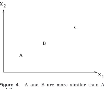
num-ber of xj with respect to xi. Figures 4
and 5 give an example. In Figure 4, the nearest neighbor of A is B, and B’s nearest neighbor is A. So, NN~A, B! 5
NN~B, A! 5 1 and the MND between A and B is 2. However, NN~B, C! 5 1 but NN~C, B! 5 2, and therefore MND~B, C! 5 3. Figure 5 was ob-tained from Figure 4 by adding three new points D, E, and F. Now MND~B, C! 5 3 (as before), but MND~A, B! 5 5. The MND between A and B has in-creased by introducing additional points, even though A and B have not moved. The MND is not a metric (it does not satisfy the triangle inequality [Zhang 1995]). In spite of this, MND has been successfully applied in several clustering applications [Gowda and Di-day 1992]. This observation supports the viewpoint that the dissimilarity does not need to be a metric.
Watanabe’s theorem of the ugly duck-ling [Watanabe 1985] states:
“Insofar as we use a finite set of predicates that are capable of dis-tinguishing any two objects con-sidered, the number of predicates shared by any two such objects is constant, independent of the choice of objects.”
This implies that it is possible to make any two arbitrary patterns equally similar by encoding them with a sufficiently large number of features. As a consequence, any two arbitrary pat-terns are equally similar, unless we use some additional domain information. For example, in the case of conceptual clustering [Michalski and Stepp 1983], the similarity between xi and xj is
de-fined as
s~xi,xj! 5f~xi,xj,#,%!,
where#is a set of pre-defined concepts.
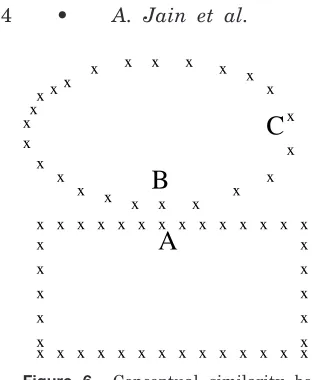
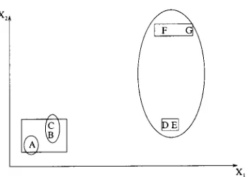
This notion is illustrated with the help of Figure 6. Here, the Euclidean dis-tance between points A and B is less than that between B and C. However, B and C can be viewed as “more similar” than A and B because B and C belong to the same concept (ellipse) and A belongs to a different concept (rectangle). The conceptual similarity measure is the most general similarity measure. We A
B
C
X X
1 2
Figure 4. A and B are more similar than A and C.
A
B
C
X X
1 2
D F E
discuss several pragmatic issues associ-ated with its use in Section 5.
5. CLUSTERING TECHNIQUES
Different approaches to clustering data can be described with the help of the hierarchy shown in Figure 7 (other tax-onometric representations of clustering methodology are possible; ours is based on the discussion in Jain and Dubes [1988]). At the top level, there is a dis-tinction between hierarchical and parti-tional approaches (hierarchical methods produce a nested series of partitions, while partitional methods produce only one).
The taxonomy shown in Figure 7 must be supplemented by a discussion of cross-cutting issues that may (in principle) affect all of the different ap-proaches regardless of their placement in the taxonomy.
—Agglomerative vs. divisive: This as-pect relates to algorithmic structure and operation. An agglomerative ap-proach begins with each pattern in a distinct (singleton) cluster, and suc-cessively merges clusters together un-til a stopping criterion is satisfied. A divisive method begins with all pat-terns in a single cluster and performs splitting until a stopping criterion is met.
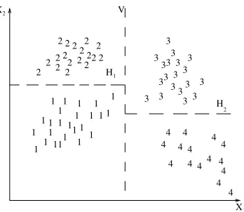
—Monotheticvs. polythetic: This aspect relates to the sequential or simulta-neous use of features in the clustering process. Most algorithms are polythe-tic; that is, all features enter into the computation of distances between patterns, and decisions are based on those distances. A simple monothetic algorithm reported in Anderberg [1973] considers features sequentially to divide the given collection of pat-terns. This is illustrated in Figure 8. Here, the collection is divided into two groups using featurex1; the verti-cal broken line V is the separating line. Each of these clusters is further divided independently using feature x2, as depicted by the broken linesH1
andH2. The major problem with this
algorithm is that it generates2d
clus-ters where d is the dimensionality of the patterns. For large values of d (d . 100 is typical in information re-trieval applications [Salton 1991]), the number of clusters generated by this algorithm is so large that the data set is divided into uninterest-ingly small and fragmented clusters.
—Hard vs. fuzzy: A hard clustering al-gorithm allocates each pattern to a single cluster during its operation and in its output. A fuzzy clustering method assigns degrees of member-ship in several clusters to each input pattern. A fuzzy clustering can be converted to a hard clustering by as-signing each pattern to the cluster with the largest measure of member-ship.
—Deterministic vs. stochastic: This is-sue is most relevant to partitional approaches designed to optimize a squared error function. This optimiza-tion can be accomplished using tradi-tional techniques or through a ran-dom search of the state space consisting of all possible labelings.
—Incremental vs. non-incremental: This issue arises when the pattern set x x x x x x x x x x x x x x
to be clustered is large, and con-straints on execution time or memory space affect the architecture of the algorithm. The early history of clus-tering methodology does not contain many examples of clustering algo-rithms designed to work with large data sets, but the advent of data min-ing has fostered the development of clustering algorithms that minimize the number of scans through the tern set, reduce the number of pat-terns examined during execution, or reduce the size of data structures used in the algorithm’s operations.
A cogent observation in Jain and Dubes [1988] is that the specification of an algorithm for clustering usually leaves considerable flexibilty in imple-mentation.
5.1 Hierarchical Clustering Algorithms The operation of a hierarchical cluster-ing algorithm is illustrated uscluster-ing the two-dimensional data set in Figure 9. This figure depicts seven patterns la-beled A, B, C, D, E, F, and G in three clusters. A hierarchical algorithm yields a dendrogram representing the nested grouping of patterns and similarity lev-els at which groupings change. A den-drogram corresponding to the seven
points in Figure 9 (obtained from the single-link algorithm [Jain and Dubes 1988]) is shown in Figure 10. The den-drogram can be broken at different lev-els to yield different clusterings of the data.
Most hierarchical clustering algo-rithms are variants of the single-link [Sneath and Sokal 1973], complete-link [King 1967], and minimum-variance [Ward 1963; Murtagh 1984] algorithms. Of these, the single-link and complete-link algorithms are most popular. These two algorithms differ in the way they characterize the similarity between a pair of clusters. In the single-link method, the distance between two clus-Clustering
Figure 7. A taxonomy of clustering approaches.
X
ters is the minimum of the distances between all pairs of patterns drawn from the two clusters (one pattern from the first cluster, the other from the sec-ond). In the complete-link algorithm, the distance between two clusters is the maximum of all pairwise distances
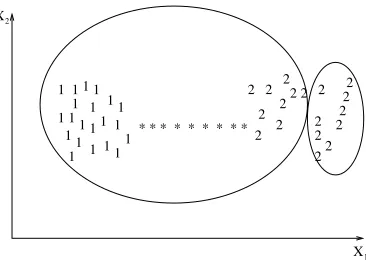
be-tween patterns in the two clusters. In either case, two clusters are merged to form a larger cluster based on minimum distance criteria. The complete-link al-gorithm produces tightly bound or com-pact clusters [Baeza-Yates 1992]. The single-link algorithm, by contrast, suf-fers from a chaining effect [Nagy 1968]. It has a tendency to produce clusters that are straggly or elongated. There are two clusters in Figures 12 and 13 separated by a “bridge” of noisy pat-terns. The single-link algorithm pro-duces the clusters shown in Figure 12, whereas the complete-link algorithm ob-tains the clustering shown in Figure 13. The clusters obtained by the complete-link algorithm are more compact than those obtained by the single-link algo-rithm; the cluster labeled 1 obtained using the single-link algorithm is elon-gated because of the noisy patterns la-beled “*”. The single-link algorithm is more versatile than the complete-link algorithm, otherwise. For example, the single-link algorithm can extract the concentric clusters shown in Figure 11, but the complete-link algorithm cannot. However, from a pragmatic viewpoint, it has been observed that the complete-link algorithm produces more useful hi-erarchies in many applications than the single-link algorithm [Jain and Dubes 1988].
Agglomerative Single-Link Clus-tering Algorithm
(1) Place each pattern in its own clus-ter. Construct a list of interpattern distances for all distinct unordered pairs of patterns, and sort this list in ascending order.
(2) Step through the sorted list of tances, forming for each distinct dis-similarity value dk a graph on the
patterns where pairs of patterns closer than dk are connected by a
graph edge. If all the patterns are members of a connected graph, stop. Otherwise, repeat this step.
X
A B
C D E
F G
Cluster1 Cluster2
Cluster3 X
1 2
Figure 9. Points falling in three clusters.
A B C D E F G
S i m
i l a r i t y
Figure 10. The dendrogram obtained using the single-link algorithm.
X Y
1 1
1
1
1
1 1
1 1
2
2
2 2 2 2
(3) The output of the algorithm is a nested hierarchy of graphs which can be cut at a desired dissimilarity level forming a partition (clustering) identified by simply connected com-ponents in the corresponding graph.
Agglomerative Complete-Link Clus-tering Algorithm
(1) Place each pattern in its own clus-ter. Construct a list of interpattern distances for all distinct unordered pairs of patterns, and sort this list in ascending order.
(2) Step through the sorted list of tances, forming for each distinct dis-similarity value dk a graph on the
patterns where pairs of patterns closer than dk are connected by a
graph edge. If all the patterns are members of a completely connected graph, stop.
(3) The output of the algorithm is a nested hierarchy of graphs which can be cut at a desired dissimilarity level forming a partition (clustering) identified by completely connected components in the corresponding graph.
Hierarchical algorithms are more ver-satile than partitional algorithms. For example, the single-link clustering algo-rithm works well on data sets contain-ing non-isotropic clusters including
well-separated, chain-like, and concen-tric clusters, whereas a typical parti-tional algorithm such as the k-means algorithm works well only on data sets having isotropic clusters [Nagy 1968]. On the other hand, the time and space complexities [Day 1992] of the parti-tional algorithms are typically lower than those of the hierarchical algo-rithms. It is possible to develop hybrid algorithms [Murty and Krishna 1980] that exploit the good features of both categories.
Hierarchical Agglomerative Clus-tering Algorithm
(1) Compute the proximity matrix con-taining the distance between each pair of patterns. Treat each pattern as a cluster.
(2) Find the most similar pair of clus-ters using the proximity matrix. Merge these two clusters into one cluster. Update the proximity ma-trix to reflect this merge operation.
(3) If all patterns are in one cluster, stop. Otherwise, go to step 2.
Based on the way the proximity matrix is updated in step 2, a variety of ag-glomerative algorithms can be designed. Hierarchical divisive algorithms start with a single cluster of all the given objects and keep splitting the clusters based on some criterion to obtain a par-tition of singleton clusters.
1 1
Figure 12. A single-link clustering of a pattern set containing two classes (1 and 2) connected by a chain of noisy patterns (*).
1 1
5.2 Partitional Algorithms
A partitional clustering algorithm ob-tains a single partition of the data in-stead of a clustering structure, such as the dendrogram produced by a hierar-chical technique. Partitional methods have advantages in applications involv-ing large data sets for which the con-struction of a dendrogram is computa-tionally prohibitive. A problem accompanying the use of a partitional algorithm is the choice of the number of desired output clusters. A seminal pa-per [Dubes 1987] provides guidance on this key design decision. The partitional techniques usually produce clusters by optimizing a criterion function defined either locally (on a subset of the pat-terns) or globally (defined over all of the patterns). Combinatorial search of the set of possible labelings for an optimum value of a criterion is clearly computa-tionally prohibitive. In practice, there-fore, the algorithm is typically run mul-tiple times with different starting states, and the best configuration ob-tained from all of the runs is used as the output clustering.
5.2.1 Squared Error Algorithms. The most intuitive and frequently used criterion function in partitional cluster-ing techniques is the squared error cri-terion, which tends to work well with isolated and compact clusters. The squared error for a clustering + of a
pattern set- (containingK clusters) is
e2~-,+! 5
O
j51K
O
i51
nj
ixi ~j!2
cji2,
where xi~j!is theith pattern belonging to
the jth cluster and c
j is the centroid of
thejth cluster.
Thek-means is the simplest and most commonly used algorithm employing a squared error criterion [McQueen 1967]. It starts with a random initial partition and keeps reassigning the patterns to clusters based on the similarity between the pattern and the cluster centers until
a convergence criterion is met (e.g., there is no reassignment of any pattern from one cluster to another, or the squared error ceases to decrease signifi-cantly after some number of iterations). The k-means algorithm is popular be-cause it is easy to implement, and its time complexity isO~n!, where n is the number of patterns. A major problem with this algorithm is that it is sensitive to the selection of the initial partition and may converge to a local minimum of the criterion function value if the initial partition is not properly chosen. Figure 14 shows seven two-dimensional pat-terns. If we start with patterns A, B, and C as the initial means around which the three clusters are built, then we end up with the partition {{A}, {B, C}, {D, E, F, G}} shown by ellipses. The squared error criterion value is much larger for this partition than for the best partition {{A, B, C}, {D, E}, {F, G}} shown by rectangles, which yields the global minimum value of the squared error criterion function for a clustering containing three clusters. The correct three-cluster solution is obtained by choosing, for example, A, D, and F as the initial cluster means.
Squared Error Clustering Method (1) Select an initial partition of the pat-terns with a fixed number of clus-ters and cluster cenclus-ters.
(2) Assign each pattern to its closest cluster center and compute the new cluster centers as the centroids of the clusters. Repeat this step until convergence is achieved, i.e., until the cluster membership is stable. (3) Merge and split clusters based on
some heuristic information, option-ally repeating step 2.
k-Means Clustering Algorithm
(2) Assign each pattern to the closest cluster center.
(3) Recompute the cluster centers using the current cluster memberships.
(4) If a convergence criterion is not met, go to step 2. Typical convergence criteria are: no (or minimal) reas-signment of patterns to new cluster centers, or minimal decrease in squared error.
Several variants [Anderberg 1973] of the k-means algorithm have been re-ported in the literature. Some of them attempt to select a good initial partition so that the algorithm is more likely to find the global minimum value.
Another variation is to permit split-ting and merging of the resulsplit-ting clus-ters. Typically, a cluster is split when its variance is above a pre-specified threshold, and two clusters are merged when the distance between their cen-troids is below another pre-specified threshold. Using this variant, it is pos-sible to obtain the optimal partition starting from any arbitrary initial parti-tion, provided proper threshold values are specified. The well-known ISO-DATA [Ball and Hall 1965] algorithm employs this technique of merging and splitting clusters. If ISODATA is given the “ellipse” partitioning shown in Fig-ure 14 as an initial partitioning, it will produce the optimal three-cluster
parti-tioning. ISODATA will first merge the clusters {A} and {B,C} into one cluster because the distance between their cen-troids is small and then split the cluster {D,E,F,G}, which has a large variance, into two clusters {D,E} and {F,G}.
Another variation of the k-means al-gorithm involves selecting a different criterion function altogether. The dy-namic clustering algorithm (which per-mits representations other than the centroid for each cluster) was proposed in Diday [1973], and Symon [1977] and describes a dynamic clustering ap-proach obtained by formulating the clustering problem in the framework of maximum-likelihood estimation. The regularized Mahalanobis distance was used in Mao and Jain [1996] to obtain hyperellipsoidal clusters.
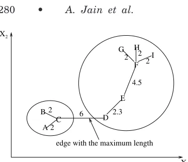
5.2.2 Graph-Theoretic Clustering. The best-known graph-theoretic divisive clustering algorithm is based on con-struction of the minimal spanning tree (MST) of the data [Zahn 1971], and then deleting the MST edges with the largest lengths to generate clusters. Figure 15 depicts the MST obtained from nine two-dimensional points. By breaking the link labeled CD with a length of 6 units (the edge with the maximum Eu-clidean length), two clusters ({A, B, C} and {D, E, F, G, H, I}) are obtained. The second cluster can be further divided into two clusters by breaking the edge EF, which has a length of 4.5 units.
The hierarchical approaches are also related to graph-theoretic clustering. Single-link clusters are subgraphs of the minimum spanning tree of the data [Gower and Ross 1969] which are also the connected components [Gotlieb and Kumar 1968]. Complete-link clusters are maximal complete subgraphs, and are related to the node colorability of graphs [Backer and Hubert 1976]. The maximal complete subgraph was consid-ered the strictest definition of a cluster in Augustson and Minker [1970] and Raghavan and Yu [1981]. A graph-ori-ented approach for non-hierarchical structures and overlapping clusters is
presented in Ozawa [1985]. The Delau-nay graph (DG) is obtained by connect-ing all the pairs of points that are Voronoi neighbors. The DG contains all the neighborhood information contained in the MST and the relative neighbor-hood graph (RNG) [Toussaint 1980].
5.3 Mixture-Resolving and Mode-Seeking Algorithms
The mixture resolving approach to clus-ter analysis has been addressed in a number of ways. The underlying as-sumption is that the patterns to be clus-tered are drawn from one of several distributions, and the goal is to identify the parameters of each and (perhaps) their number. Most of the work in this area has assumed that the individual components of the mixture density are Gaussian, and in this case the parame-ters of the individual Gaussians are to be estimated by the procedure. Tradi-tional approaches to this problem in-volve obtaining (iteratively) a maximum likelihood estimate of the parameter vectors of the component densities [Jain and Dubes 1988].
More recently, the Expectation Maxi-mization (EM) algorithm (a general-purpose maximum likelihood algorithm [Dempster et al. 1977] for missing-data problems) has been applied to the prob-lem of parameter estimation. A recent book [Mitchell 1997] provides an
acces-sible description of the technique. In the EM framework, the parameters of the component densities are unknown, as are the mixing parameters, and these are estimated from the patterns. The EM procedure begins with an initial estimate of the parameter vector and iteratively rescores the patterns against the mixture density produced by the parameter vector. The rescored patterns are then used to update the parameter estimates. In a clustering context, the scores of the patterns (which essentially measure their likelihood of being drawn from particular components of the mix-ture) can be viewed as hints at the class of the pattern. Those patterns, placed (by their scores) in a particular compo-nent, would therefore be viewed as be-longing to the same cluster.
Nonparametric techniques for densi-ty-based clustering have also been de-veloped [Jain and Dubes 1988]. Inspired by the Parzen window approach to non-parametric density estimation, the cor-responding clustering procedure searches for bins with large counts in a multidimensional histogram of the put pattern set. Other approaches in-clude the application of another parti-tional or hierarchical clustering algorithm using a distance measure based on a nonparametric density esti-mate.
5.4 Nearest Neighbor Clustering
Since proximity plays a key role in our intuitive notion of a cluster, nearest-neighbor distances can serve as the ba-sis of clustering procedures. An itera-tive procedure was proposed in Lu and Fu [1978]; it assigns each unlabeled pattern to the cluster of its nearest la-beled neighbor pattern, provided the distance to that labeled neighbor is be-low a threshold. The process continues until all patterns are labeled or no addi-tional labelings occur. The mutual neighborhood value (described earlier in the context of distance computation) can also be used to grow clusters from near neighbors.
X B
A C
D E
F
G H
I
edge with the maximum length 2
2
6 2.3
4.5
2 2 2
X2
1
5.5 Fuzzy Clustering
Traditional clustering approaches gen-erate partitions; in a partition, each pattern belongs to one and only one cluster. Hence, the clusters in a hard clustering are disjoint. Fuzzy clustering extends this notion to associate each pattern with every cluster using a mem-bership function [Zadeh 1965]. The out-put of such algorithms is a clustering, but not a partition. We give a high-level partitional fuzzy clustering algorithm below.
Fuzzy Clustering Algorithm
(1) Select an initial fuzzy partition of the N objects into K clusters by selecting the N 3 K membership matrix U. An element uij of this
matrix represents the grade of mem-bership of object xi in cluster cj.
Typically, uij [ @0,1#.
(2) Using U, find the value of a fuzzy criterion function, e.g., a weighted squared error criterion function, as-sociated with the corresponding par-tition. One possible fuzzy criterion function is
E2~-,U! 5
O
i51
N
O
k51
K
uijixi2cki2,
where ck 5 ( i51
N
uikxi is the kth fuzzy
cluster center.
Reassign patterns to clusters to re-duce this criterion function value and recompute U.
(3) Repeat step 2 until entries in U do not change significantly.
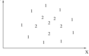
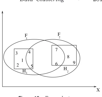
In fuzzy clustering, each cluster is a fuzzy set of all the patterns. Figure 16 illustrates the idea. The rectangles en-close two “hard” clusters in the data: H1 5 $1,2,3,4,5% and H2 5 $6,7,8,9%.
A fuzzy clustering algorithm might pro-duce the two fuzzy clusters F1 and F2
depicted by ellipses. The patterns will
have membership values in [0,1] for each cluster. For example, fuzzy cluster F1 could be compactly described as
$~1,0.9!,~2,0.8!,~3,0.7!,~4,0.6!,~5,0.55!,
~6,0.2!,~7,0.2!,~8,0.0!,~9,0.0!%
andF2 could be described as
$~1,0.0!,~2,0.0!,~3,0.0!,~4,0.1!,~5,0.15!,
~6,0.4!,~7,0.35!,~8,1.0!,~9,0.9!%
The ordered pairs~i, mi! in each cluster
represent the ith pattern and its mem-bership value to the cluster mi. Larger
membership values indicate higher con-fidence in the assignment of the pattern to the cluster. A hard clustering can be obtained from a fuzzy partition by thresholding the membership value.
Fuzzy set theory was initially applied to clustering in Ruspini [1969]. The book by Bezdek [1981] is a good source for material on fuzzy clustering. The most popular fuzzy clustering algorithm is the fuzzy c-means (FCM) algorithm. Even though it is better than the hard k-means algorithm at avoiding local minima, FCM can still converge to local minima of the squared error criterion. The design of membership functions is the most important problem in fuzzy clustering; different choices include X Y
1 2
3 4
5 6
7 8
9
H H2
F F
1
1 2
those based on similarity decomposition and centroids of clusters. A generaliza-tion of the FCM algorithm was proposed by Bezdek [1981] through a family of objective functions. A fuzzyc-shell algo-rithm and an adaptive variant for de-tecting circular and elliptical bound-aries was presented in Dave [1992].
5.6 Representation of Clusters
In applications where the number of classes or clusters in a data set must be discovered, a partition of the data set is the end product. Here, a partition gives an idea about the separability of the data points into clusters and whether it is meaningful to employ a supervised classifier that assumes a given number of classes in the data set. However, in many other applications that involve decision making, the resulting clusters have to be represented or described in a compact form to achieve data abstrac-tion. Even though the construction of a cluster representation is an important step in decision making, it has not been examined closely by researchers. The notion of cluster representation was in-troduced in Duran and Odell [1974] and was subsequently studied in Diday and Simon [1976] and Michalski et al. [1981]. They suggested the following representation schemes:
(1) Represent a cluster of points by their centroid or by a set of distant points in the cluster. Figure 17 de-picts these two ideas.
(2) Represent clusters using nodes in a classification tree. This is illus-trated in Figure 18.
(3) Represent clusters by using conjunc-tive logical expressions. For example, the expression @X1 . 3#@X2 , 2# in
Figure 18 stands for the logical state-ment ‘X1 is greater than 3’and’X2 is
less than 2’.
Use of the centroid to represent a cluster is the most popular scheme. It works well when the clusters are com-pact or isotropic. However, when the clusters are elongated or non-isotropic, then this scheme fails to represent them properly. In such a case, the use of a collection of boundary points in a clus-ter captures its shape well. The number of points used to represent a cluster should increase as the complexity of its shape increases. The two different rep-resentations illustrated in Figure 18 are equivalent. Every path in a classifica-tion tree from the root node to a leaf node corresponds to a conjunctive state-ment. An important limitation of the typical use of the simple conjunctive concept representations is that they can describe only rectangular or isotropic clusters in the feature space.
Data abstraction is useful in decision making because of the following:
(1) It gives a simple and intuitive de-scription of clusters which is easy for human comprehension. In both conceptual clustering [Michalski
X X
By Three Distant Points By The Centroid
* *
* *
* *
* *
*
* *
*
*
*
1
X2 X2
1
and Stepp 1983] and symbolic clus-tering [Gowda and Diday 1992] this representation is obtained without using an additional step. These al-gorithms generate the clusters as well as their descriptions. A set of fuzzy rules can be obtained from fuzzy clusters of a data set. These rules can be used to build fuzzy clas-sifiers and fuzzy controllers.
(2) It helps in achieving data compres-sion that can be exploited further by a computer [Murty and Krishna 1980]. Figure 19(a) shows samples belonging to two chain-like clusters labeled 1 and 2. A partitional clus-tering like the k-means algorithm cannot separate these two struc-tures properly. The single-link algo-rithm works well on this data, but is computationally expensive. So a hy-brid approach may be used to ex-ploit the desirable properties of both these algorithms. We obtain 8 sub-clusters of the data using the (com-putationally efficient)k-means algo-rithm. Each of these subclusters can be represented by their centroids as shown in Figure 19(a). Now the sin-gle-link algorithm can be applied on these centroids alone to cluster them into 2 groups. The resulting groups are shown in Figure 19(b). Here, a data reduction is achieved
by representing the subclusters by their centroids.
(3) It increases the efficiency of the de-cision making task. In a cluster-based document retrieval technique [Salton 1991], a large collection of documents is clustered and each of the clusters is represented using its centroid. In order to retrieve docu-ments relevant to a query, the query is matched with the cluster cen-troids rather than with all the docu-ments. This helps in retrieving rele-vant documents efficiently. Also in several applications involving large data sets, clustering is used to per-form indexing, which helps in effi-cient decision making [Dorai and Jain 1995].
5.7 Artificial Neural Networks for Clustering
Artificial neural networks (ANNs) [Hertz et al. 1991] are motivated by biological neural networks. ANNs have been used extensively over the past three decades for both classification and clustering [Sethi and Jain 1991; Jain and Mao 1994]. Some of the features of the ANNs that are important in pattern clustering are: Using Nodes in a Classification Tree
Using Conjunctive Statements X2
(1) ANNs process numerical vectors and so require patterns to be represented using quantitative features only.
(2) ANNs are inherently parallel and distributed processing architec-tures.
(3) ANNs may learn their interconnec-tion weights adaptively [Jain and Mao 1996; Oja 1982]. More specifi-cally, they can act as pattern nor-malizers and feature selectors by appropriate selection of weights.
Competitive (or winner–take–all) neural networks [Jain and Mao 1996] are often used to cluster input data. In competitive learning, similar patterns are grouped by the network and repre-sented by a single unit (neuron). This grouping is done automatically based on data correlations. Well-known examples of ANNs used for clustering include Ko-honen’s learning vector quantization (LVQ) and self-organizing map (SOM) [Kohonen 1984], and adaptive reso-nance theory models [Carpenter and Grossberg 1990]. The architectures of these ANNs are simple: they are single-layered. Patterns are presented at the input and are associated with the out-put nodes. The weights between the in-put nodes and the outin-put nodes are iteratively changed (this is called learn-ing) until a termination criterion is sat-isfied. Competitive learning has been found to exist in biological neural net-works. However, the learning or weight update procedures are quite similar to
those in some classical clustering ap-proaches. For example, the relationship between the k-means algorithm and LVQ is addressed in Pal et al. [1993]. The learning algorithm in ART models is similar to the leader clustering algo-rithm [Moor 1988].
The SOM gives an intuitively appeal-ing two-dimensional map of the multidi-mensional data set, and it has been successfully used for vector quantiza-tion and speech recogniquantiza-tion [Kohonen 1984]. However, like its sequential counterpart, the SOM generates a sub-optimal partition if the initial weights are not chosen properly. Further, its convergence is controlled by various pa-rameters such as the learning rate and a neighborhood of the winning node in which learning takes place. It is possi-ble that a particular input pattern can fire different output units at different iterations; this brings up the stability issue of learning systems. The system is said to be stable if no pattern in the training data changes its category after a finite number of learning iterations. This problem is closely associated with the problem of plasticity, which is the ability of the algorithm to adapt to new data. For stability, the learning rate should be decreased to zero as iterations progress and this affects the plasticity. The ART models are supposed to be stable and plastic [Carpenter and Grossberg 1990]. However, ART nets are order-dependent; that is, different partitions are obtained for different or-ders in which the data is presented to the net. Also, the size and number of clusters generated by an ART net de-pend on the value chosen for the vigi-lance threshold, which is used to decide whether a pattern is to be assigned to one of the existing clusters or start a new cluster. Further, both SOM and ART are suitable for detecting only hy-perspherical clusters [Hertz et al. 1991]. A two-layer network that employs regu-larized Mahalanobis distance to extract hyperellipsoidal clusters was proposed in Mao and Jain [1994]. All these ANNs use a fixed number of output nodes 1
which limit the number of clusters that can be produced.
5.8 Evolutionary Approaches for Clustering
Evolutionary approaches, motivated by natural evolution, make use of evolu-tionary operators and a population of solutions to obtain the globally optimal partition of the data. Candidate solu-tions to the clustering problem are en-coded as chromosomes. The most com-monly used evolutionary operators are: selection, recombination, and mutation. Each transforms one or more input chromosomes into one or more output chromosomes. A fitness function evalu-ated on a chromosome determines a chromosome’s likelihood of surviving into the next generation. We give below a high-level description of an evolution-ary algorithm applied to clustering.
An Evolutionary Algorithm for Clustering
(1) Choose a random population of solu-tions. Each solution here corre-sponds to a valid k-partition of the data. Associate a fitness value with each solution. Typically, fitness is inversely proportional to the squared error value. A solution with a small squared error will have a larger fitness value.
(2) Use the evolutionary operators se-lection, recombination and mutation to generate the next population of solutions. Evaluate the fitness val-ues of these solutions.
(3) Repeat step 2 until some termina-tion conditermina-tion is satisfied.
The best-known evolutionary tech-niques are genetic algorithms (GAs) [Holland 1975; Goldberg 1989], evolu-tion strategies (ESs) [Schwefel 1981], and evolutionary programming (EP) [Fogel et al. 1965]. Out of these three approaches, GAs have been most fre-quently used in clustering. Typically, solutions are binary strings in GAs. In
GAs, a selection operator propagates so-lutions from the current generation to the next generation based on their fit-ness. Selection employs a probabilistic scheme so that solutions with higher fitness have a higher probability of get-ting reproduced.
There are a variety of recombination operators in use; crossover is the most popular. Crossover takes as input a pair of chromosomes (called parents) and outputs a new pair of chromosomes (called children or offspring) as depicted in Figure 20. In Figure 20, a single point crossover operation is depicted. It exchanges the segments of the parents across a crossover point. For example, in Figure 20, the parents are the binary strings ‘10110101’ and ‘11001110’. The segments in the two parents after the crossover point (between the fourth and fifth locations) are exchanged to pro-duce the child chromosomes. Mutation takes as input a chromosome and out-puts a chromosome by complementing the bit value at a randomly selected location in the input chromosome. For example, the string ‘11111110’ is gener-ated by applying the mutation operator to the second bit location in the string ‘10111110’ (starting at the left). Both crossover and mutation are applied with some prespecified probabilities which depend on the fitness values.
GAs represent points in the search space as binary strings, and rely on the
parent1
parent2
child1
child2
1 0 1 1 0 1 0 1
1 0 1 1 1 1 1 0
1 1 0 0 0 1 0 1 1 1 0 0 1 1 1 0
crossover point
crossover operator to explore the search space. Mutation is used in GAs for the sake of completeness, that is, to make sure that no part of the search space is left unexplored. ESs and EP differ from the GAs in solution representation and type of the mutation operator used; EP does not use a recombination operator, but only selection and mutation. Each of these three approaches have been used to solve the clustering problem by view-ing it as a minimization of the squared error criterion. Some of the theoretical issues such as the convergence of these approaches were studied in Fogel and Fogel [1994].
GAs perform a globalized search for solutions whereas most other clustering procedures perform a localized search. In a localized search, the solution ob-tained at the ‘next iteration’ of the pro-cedure is in the vicinity of the current solution. In this sense, the k-means al-gorithm, fuzzy clustering algorithms, ANNs used for clustering, various an-nealing schemes (see below), and tabu search are all localized search tech-niques. In the case of GAs, the crossover and mutation operators can produce new solutions that are completely dif-ferent from the current ones. We illus-trate this fact in Figure 21. Let us as-sume that the scalar X is coded using a 5-bit binary representation, and let S1
and S2 be two points in the
one-dimen-sional search space. The decimal values of S1 andS2 are 8 and 31, respectively.
Their binary representations are S1 5
01000 and S2 5 11111. Let us apply the single-point crossover to these strings, with the crossover site falling between the second and third most sig-nificant bits as shown below.
01!000
11!111
This will produce a new pair of points or chromosomes S3 and S4 as shown in
Figure 21. Here, S3 5 01111 and
S4 5 11000. The corresponding
deci-mal values are 15 and 24, respectively. Similarly, by mutating the most signifi-cant bit in the binary string 01111 (dec-imal 15), the binary string 11111 (deci-mal 31) is generated. These jumps, or gaps between points in successive gen-erations, are much larger than those produced by other approaches.
Perhaps the earliest paper on the use of GAs for clustering is by Raghavan and Birchand [1979], where a GA was used to minimize the squared error of a clustering. Here, each point or chromo-some represents a partition ofN objects into K clusters and is represented by a K-ary string of length N. For example, consider six patterns—A, B, C, D, E, and F—and the string 101001. This six-bit binary (K 5 2) string corresponds to placing the six patterns into two clus-ters. This string represents a two-parti-tion, where one cluster has the first, third, and sixth patterns and the second cluster has the remaining patterns. In other words, the two clusters are {A,C,F} and {B,D,E} (the six-bit binary string 010110 represents the same clus-tering of the six patterns). When there are K clusters, there are K! different chromosomes corresponding to each K-partition of the data. This increases the effective search space size by a fac-tor ofK!. Further, if crossover is applied on two good chromosomes, the resulting
f(X)
X S
S S S
1 3 4 2
X X
X
X