GLOF STUDY IN TAWANG RIVER BASIN, ARUNACHAL PRADESH, INDIA
Rupasree Panda a, Suman Kumar Padhee b, *, Subashisa Dutta c
a Department of Civil Engineering, M. Tech. Student, Indian Institute of Technology, Guwahati – [email protected] b Department of Civil Engineering, PhD. Research Scholar, Indian Institute of Technology, Guwahati - [email protected]
c Department of Civil Engineering, Professor, Indian Institute of Technology, Guwahati - [email protected]
KEY WORDS:Glacial lake outburst flood (GLOF), Landsat-8, HEC-RAS, Hydrodynamic channel routing
ABSTRACT:
Glacial lake outburst flood (GLOF) is one of the major unexpected hazards in the high mountain regions susceptible to climate change. The Tawang river basin in Arunachal Pradesh is an unexplored region in the Eastern Himalayas, which is impending to produce several upcoming hydro-electric projects (HEP). The main source of the river system is the snow melt in the Eastern Himalayas, which is composed of several lakes located at the snout of the glacier dammed by the lateral or end moraine. These lakes might prove as potential threat to the future scenario as they have a tendency to produce flash flood with large quantity of sediment load during outbursts. This study provides a methodology to detect the potential lakes as a danger to the HEP sites in the basin, followed by quantification of volume of discharge from the potential lake and prediction of hydrograph at the lake site. The remote location of present lakes induced the use of remote sensing data, which was fulfilled by Landsat-8 satellite imagery with least cloud coverage. Suitable reflectance bands on the basis of spectral responses were used to produce informational layers (NDWI, Potential snow cover map, supervised classification map) in GIS environment for discriminating different land features. The product obtained from vector overlay operation of these layers; representing possible water area, was further utilized in combination with Google earth to identify the lakes within the watershed. Finally those identified lakes were detected as potentially dangerous lakes based on the criteria of elevation, area, proximity from streamline, slope and volume of water held. HEC-RAS simulation model was used with cross sections from Google Earth and field survey as input to simulate dam break like situation; hydrodynamic channel routing of the outburst hydrograph along river reach was carried out to get the GLOF hydrograph at the project sites. It was concluded from the results that, the assessed GLOF would be a lead for the qualitative approximation of the amount of bed load transported along the river reach and thus hydropower project sites.
1. INTRODUCTION
1.1 Glacial Lakes and its Types
The majority of glacial lakes are found by the accumulation of huge amount of water from snow and ice cover melting and dammed by unstable moraines in the Himalayan region. Glacial lakes can be classified into several types according to their position relative to the glacier and damming mechanism. Glacial lakes can be of various types such as pro glacial, en glacial, sub glacial, supra glacial and moraine dammed lakes. moraine dammed lakes are mainly composed of unsorted, unconsolidated boulders, gravels, sands, clays and are frequently reinforced by frozen cores, that are likely to melt. Sometimes these moraine dammed lakes located at the snout of the glacier are mainly dammed by the lateral or end moraine, where there is high tendency of breaching. In addition to structural instability, they may hold a large quantity of water, ultimately leads to Breaching and the instantaneous discharge of water from the lake, called flash flood.
1.1.1 Moraine Dammed Lake: Under the influence of retreating of glacier, assorted accumulation of soil, rock and materials that carried away from the glacier takes place, eventually leads to formation of lateral and end moraines. As the name suggests, end moraines are formed at furthermost limit reached by a glacier and lateral moraines are formed by the sides of glacier. These moraine dammed lakes are mainly located at the snout of glacier and formed by the damming mechanism of lateral and end
moraines, i.e., both the lateral and end moraines may work as dams. The moraine acts as an unstable dam to water melting from the glacier. As retreats and advances of valley glaciers takes place, the lowest portion of glacier gradually bounded by lateral and end moraines in the mountain valley and in due course the formation of moraine-dammed glacial lake starts. Such glacial lakes are essentially ephemeral and are not stable from the point of view of the life of glaciers. Generally, moraine dammed lakes pose a threat in the basin. Most of the moraine dams and moraine-dammed glacial lakes have a record of recurring outburst activity. The cyclical outburst activity ends when the moraine dam is damaged by the outburst floods to the extent that it can no longer hold water. As glaciers retreat, the cyclic outburst activity may move up glacier to newly formed moraine dams and moraine-dammed lakes (Clague 2003).
gradually or abruptly decrease to normal levels once the water source is exhausted. The peak flow of GLOF is directly related to lake volume, dam height and width, dam material composition, failure mechanism, downstream topography, and sediment availability. GLOF have direct impact on the commissioned hydropower projects and the population living in the downstream area.
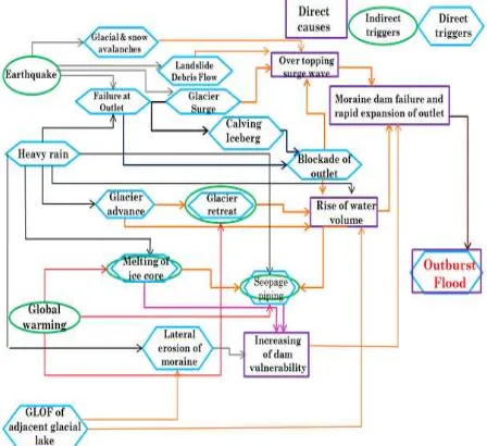
Figure 1: Causes for GLOF and triggers for moraines to fail
2. MATERIALS AND METHODS
2.1 Study Area
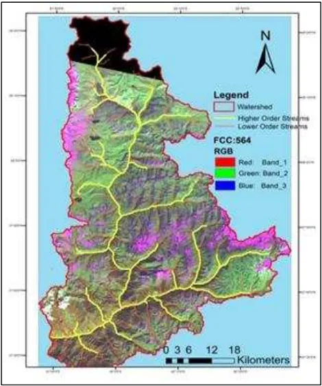
Figure 2: Study area map
The Tawang region in western parts of Arunachal Pradesh, India, is sandwiched between Bhutan in west and China in North (Figure 2). The total geographical area of the study region is approximately 3447 km2, with spatial extent of Longitude 91º45'2.303"E to 92º29'17.586"E and Latitude 27º28'20.611"N to 28º22'42.051"N (Figure 2). The main river line in the Study area is Tawang Chu, which has two perennial tributaries; Nyukcharong Chu and Mago Chu originating in China, Arunachal Pradesh and then forms two sub catchments namely Nyukcharong Chu catchment and Mago Chu catchment respectively. Ultimately Tawang Chu further extends to join with Brahmaputra in Assam. Tawang river basin is an unexplored region in the Eastern Himalayas, which is impending to produce several upcoming hydro-electric projects (HEP). Two of the major HEPs, Mago Chu and Nyukcharong Chu are selected in the present study.
2.2 Data Description
2.2.1 Satellite Data: Medium to high resolution multispectral and multi date satellite images were used for and delineation of watershed and lake identification process in the study.
(a) DEM (Digital Elevation Model): NASA (National
Aeronautics and Space Administration) has provided 90 m (3-arc second) DEMs for about 80% of the globe under the program SRTM (Shuttle Radar Topographic Mission). The DEM data is highly useful for delineation of catchment and extracting catchment parameters such as slope, area, contours etc. at a spatial extent. Considering the fact that the catchment area is divided in Indian and Chinese premises, the 90 m SRTM DEM was used for delineating the catchment.
(b) Landsat-8: It carries two push broom sensors; OLI (Operational land imager) and TIRS (Thermal infrared sensors). Landsat-8 data products are level-1 (Ortho rectified data product). The standard level-1 data products were downloaded from Landsat look viewer (http://landsatlook.usgs.gov/). The OLI sensor collects data for 9 short wave spectral bands over a 185 km of swath with a 30 m spatial resolution for all bands except a 15 m panchromatic band. The TIRS collects data for two thermal bands with 100 m resolution over a 185 km of swath. TIRS bands 10 and 11 collects data at 100 m and resampled to 30 m to match OLI multispectral bands. OLI level-1 data products use a 16-bit numbers representing pixel value, which is very sensitive to the small changes of the land radiance and reflectance. Fortunately the Landsat-8 scenes chosen for this study were found to have maximum cloud cover of 9%.
2.2.3 Field Data: The cross sectional data collected with the help of a Total station at different stages along the river flow, was also used. The field survey was conducted mainly at the proposed HEP site and up to the accessible upstream. Practically, the cross sections along the river line up to lake were not approachable due to which Google Earth and SRTM DEM were utilized for getting out the same. The cross section data was an essential input for hydrodynamic simulation. The requirement of the hydrodynamic model for distance of intervals between two consecutive cross sections was ranging from 500 m to 3000 m which was maintained accordingly.
2.3 Methodology
The methodology can be divided into two parts (Figure 3). The first part includes identification of glacial lakes and selection of lake potentially dangerous (critical lake) to HEPs in the study area. It is followed by the second part, estimation of GLOF at the HEP sites in the basin.
2.3.1 Identification Critical Lakes: It comprises of three parts; firstly, pre-processing of the satellite data for delineation of watershed and to draw out inferences from various image based reflectance, secondly identification of glacial lakes present in the study area, and the third part is vulnerability analysis of identified lakes for detecting the critical lake as a potential threat for occurrence of GLOF.
effects caused by both solar angle and the atmosphere. The radiance sensed in the Landsat-8 low and high gain thermal bands were converted to TOA brightness temperature (i.e., assuming unit surface emissivity). Landsat-8 OLI multispectral bands (1-7) were converted from DN to reflectance for further image based analysis. Unlike the pre-processing conducted for OLI bands, the TIRS bands (10 and 11) were converted from DN to radiance and then radiance to brightness temperature.
Figure 3: Flow diagram of the method for this study
Flow directions and flow accumulation maps were generated from SRTM-DEM using D8 flow direction method in which each pixel discharges into one of its eight neighbouring direction having steepest descent. The flow directions were determined by identifying the neighbouring cell which has the highest positive distance weighted drop. Flow accumulation is determined as the sum of the flow accumulation values of the neighbouring cells which flow into it. The streams were classified to various sub-catchments which together formed the sub-catchments of the main river course
(b) Identification of Glacial lakes: A semiautomatic 4 step screening approach was adopted for the identification of glacial (Figure 4). The steps can be segregated as: (i) Use of spectral water Index for delineating water features, (ii) Object based Semi-automatic procedure for distinguishing snow region and no snow region, (iii) Supervised classification for identification of various spectral classes that are present in the study area, (iv)Combination of above three approaches for identification of final glacial lakes.
The Normalized difference water index (NDWI) is derived from band rationing and normalization of the spectral bands (Equation 1). The design of Spectral Water Index was based on the fact that water absorbs energy at Near-Infrared (NIR) and reflects mainly within the visible spectrum with a maximum value in the green band. The selection of NIR and Green bands was decided for water detection after testing available Landsat-8 bands for quite a few methods like rationing with different band combinations. NDSI (Normalized difference snow index) was used to generate snow cover for the study basin. The NDSI was calculated as in equation (2). snow layer is as shown in Figure 5.
A False color composite FCC (5,6,4) was created considering the spectral characteristics of Landsat-8 bands (Figure 6); Band-5 (Near infrared) is especially important for ecology because healthy plants reflect it, in contrasts to this water body appears black and soil, vegetation appears bright. So it is a reasonable band for defining land and water interface. Band -6 (Short wave infrared - 1) creates contrasts between wet earth and dry earth and have a distinct spectral characteristics for geology i.e. rocks and soils. This band is preferred over the use of SWIR-2 because of its characteristics of better response to wet targets, as compared to SWIR-2; Band-4 (Red) can be used to discriminate wet features from others as the absorption of radiation in this region is pretty high due to which its response to a wet feature on earth surface is low. Supervised classification method on FCC (5,6,4) was performed. It is generally preferred when a few features are to be identified. Initially the training area was created as area of interest. Perception of the training areas was based on visual interpretation which takes care of all kinds of information like size of object, shape of object, shadow effect, tone, colour, texture, pattern and association of various spectral covers. Each pixel is assigned to the class for which it has the highest probability of membership. Supervised classification considers the mean and covariance of training set as basic marks for classification.
Figure 4. Procedure for identification of glacial lakes from Landsat-8 data.
Figure 6: False colour composite (5,6,4) of the study area.
Based on the interpretation from NDWI, NDSI and FCC (5,6,4), it was decided whether to proceed with a final approach that combines the results from all the three approaches or not. This kind of approach has the capability to strengthen the possibility of water identification.
(c) Vulnerability analysis: In order to assess the hazard from the glacial lakes, it is essential to systematically categories the glacial lakes having no risk, low risk or high risk. The lakes categorized as high risk must be studied further for risk assessment due to potential glacial lake outburst flood. The criterion for the analysis was considered for the following parameters as in Table 1 and interpretation scores are presented in Table 2.
Area
Larger area means more volume of water it will hold which will evolve into high discharge at the downstream
Slope
Gentle slope >> lower depletion of snow cover
Moderate slope >> faster depletion of snow cover
Stream Order Ordering of the stream is based on the degree of branching
Proximity
It is possible that a lake is not located on a stream, yet its proximity to a stream might make it vulnerable, so buffer of 500 m was analysed.
Elevation More prone to receive water from glacier retreat
OVERALL Sum of weights of all the attributes
Table 1. Criterion for the vulnerability analysis.
The overall vulnerability score is the sum of weights of all the attributes i.e. Overall Vulnerability weight = Area Weight + Slope Weight + Stream order Weight + Proximity Weight +
Elevation Weight. Analysis of the weights shows that the score may vary from 4 to10. Hence the criterion was used to specify the vulnerability of the lakes as shown in Table 1.
Table 2. Interpretation of score in terms of vulnerability level.
2.3.2 Estimation of GLOF: Suitable breach parameters for GLOF using DAM- BREAK simulation (unsteady flow case) was assessed. The DAM-BREAK simulation was performed in 1-D hydrodynamic mathematical model (HEC-RAS). Channel routing was done from the lakes to HEPs with flood from lake outburst as source. From these simulations, magnitude of flood peak and time of travel of peak of GLOF was estimated.
Since the simulation was assumed as an unsteady case, the parameters (volume and/or timing) of flow and stages were important for analysis. The basic theory for dynamic routing in 1-D analysis consists of two partial differential equations originally derived by (Barre De Saint Venant, 1871). The Equations are:
i) Conservation of Mass (Continuity) Equation
(∂Q/∂X) +∂ (A+ A0) / ∂t -q =0 (3)
ii) Conservation of Momentum Equation
(∂Q/∂t)+ {∂ (Q2/A)/∂X} +g A ((∂h/∂X) +Sf +Sc) =0 (4)
where, Q = Discharge in cumec, t = time in sec, q = lateral out flow in cumec/m, A0 = active flow area in m2, x = distance along waterway in m, A0=inactive storage area in m2, Sf = friction slope, Sc = expansion contraction slope, g = gravitational acceleration in m/s2.
(a) DAM BREAK Model:
Model Setup: The dam break model set up for the study was prepared which consisted by cross section at regular intervals. The cross sections were given in such a way that the highest modelled water level should not exceed the extension of these cross sections. The lakes were modelled as reservoir in HEC RAS. The point of lake location was considered as the upstream boundary of the model, where inflow hydrograph was specified.
Development (ICIMOD) guidelines and Christian Huggel’s formula (Equation 5).
International Centre for Integrated Mountain Develoment (ICIMOD) guidelines for average depth in Bhutan and Nepal:
Cirque lake - 10 m Moraine lake- 30 m Lateral moraine lake - 20 m
Blocking lake and glacier erosion lake- 40 m Trough valley lake – 25m
The Christian Huggel’s formula is basically for moraine dammed glacial lakes. Based on the data of Swiss Alps and tested for some of the glacial lakes (Raphstreng-Bhutan, TshoRolpa, Tholagi and Lower Barun-Nepal) of the Himalayas:
Other input requirements for the model are river cross-sections from lake to HEP along the river reach, and Manning’s roughness coefficient (0.055 and 0.06 for this case).
(b) Breach parameters for GLOF simulation: The breach characteristics input to dam break models are i) Final bottom width of the breach, ii) Final bottom elevation of the breach, iii) Left and right side slope of the breaching section iv) Full formation time of breach, and v) Reservoir level at time of start of breach.
Federal Energy Regulatory Commission (FERC) 1987:
2 4
Von Thun and Gillelte formula (1990):
2.5
where, Cb=18.3 for reservoir storage between 1.23 MCM to 6.17 MCM; hw = height of water above breach invert at failure in m.
Froehlich’s formula (1995 b):
0.32 0.19
where, hb= height of breach (m); K0= 1.4 for overtopping and 1.0 for piping.
(c) Boundary Conditions for Lake: For upper boundary, lake was represented in the model by elevation-cumulative volume relationship. The dam blocking of the lake was represented in the model by its crest elevation and crest length and the dam breach parameter has been specified .An initial inflow was given, whose only purpose is to run the model. For downstream boundary,
normal depth has been used as the downstream boundary for the model setup.
3. RESULTS AND DISCUSSION
3.1 Identification of Glacial Lakes
The lakes were successfully identified using the combined approach including the outputs from preparation of NDWI, potential snow layer and supervised classification. Identified lakes having an area lesser than 0.1 km2 were not considered vulnerable to floods. Hence, these lakes were not considered for further risk assessment and classification. 37 lakes in the study area were found to be satisfying this criteria. The final identified lakes with surface area greater than 0.1 km2 is presented in Figure 7.
Figure7: Identified lakes in the study area (Surface area>0.1km2)
3.2 Vulnerability Analysis
The Nyukcharong Chu stream originates from a large lake having an area approximately 22.66 km2. This lake was found in a located in a valley at an elevation of around 4749 m above MSL. The surrounding area having elevation of more than 5250 m. The lake appears to have a permanent outlet in the river Nyukcharong Chu. Thus, there are very rare chances of a GLOF event from this lake. Hence, this lake was also not considered for further study. Remaining 36 lakes were selected for further analysis for assessing the potential of causing GLOF.
Final Ranges of parameters in Identified Lakes:
Area: 0.1 km2 to 2.354 km2. Slope: 0.6% to 44.1% Stream Order: 1 to 4
Proximity: To a proximity of 500 m all the lakes were identified. Elevation: Lake center elevation was also taken into account for lake Prioritization.
The analysis show that there were 9 lakes having overall score less than or equal to 4 representing that these are not vulnerable to the GLOF. 22 lakes have score more than 5 but less than or equal to 10 showing low vulnerability. It was clear from the analysis that these lakes will not cause any significant flood due to their geographical situation in case there is any breach. The critical lakes for Nyukcharong Chu and Mago Chu catchment were found to be Lake ID-7 (27° 44' 45"N, 91° 52' 13"E) and Lake ID-20 (27°46'25.73"N, 92°18'51.73"E) respectively. The features of these two lakes were taken under consideration for GLOF simulation.
3.3 Assessment of GLOF Hydrograph at HEP
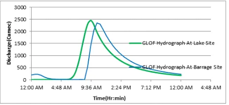
Suitable breach parameters in GLOF setup were exploited to generate hydrograph peak from Lakes ID-20, and ID-7 from DAM-BREAK simulation. Hydrodynamic routing of simulated GLOF hydrograph along the river reach was done in HEC-RAS. It was found that the peak flow takes 2 hr to reach from Lake ID-20 to HEP site at Mago Chu (Figure 8).
Figure 8. GLOF Hydrograph at Mago Chu
Similarly, analysis for Lake ID-7 showed that peak of the GLOF hydrograph, will take 1.17 hr to reach HEP site at Nyukcharong Chu (Figure 9).
Figure 9. GLOF Hydrograph at Nyukcharong Chu
3.4 Hydraulic Parameters
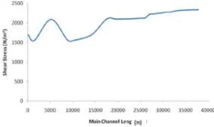
Velocity and stream power diagram for Mago Chu shows similar trend. Stream power at the middle of Mago Chu reach shows significant variation, because of narrow valley and steepest slope at that location. From the Froude’s number value in both Mago Chu and Nyukcharong Chu reaches, it can be noted that flow in both the reaches is sub critical and super critical in nature. But in Nyukcharong Chu reaches flow is predominantly super critical because of the steepest slope. Shear stress profile of both Mago Chu and Nyukcharong Chu shows significant variation. Hydraulic depth and top width profile shows wide variation because of the dynamic nature of the valley. The amount of stream power for GLOF in Mago Chu is 1,07,474.6 N/m.sec , whereas for the 100 year and 50 year return period flood the stream power comes out to be 48,889.96 N/m.sec and 43,810.49 N/m.sec respectively. Figuratively the magnitude of stream
power for GLOF is much higher than 50 year and 100 year return period flood. Figure 10 to Figure 15 shows the variation of different hydraulic parameters along the river reach of Nyukcharong Chu and Figure 16 to Figure 21 shows the same for Mago Chu.
Figure 10. Hydraulic Depth Variation along the Nyukcharong Chu Reach
Figure 11. Velocity variation along Nyukcharong Chu reach
Figure 13. Top width variation along Nyukcharong Chu reach
Figure 14. Froude number variation along Nyukcharong Chu reach
Figure 15. Shear stress variation along Nyukcharong Chu reach
Figure 16. Velocity variation along Mago Chu reach
Figure 17. Stream power variation along the Mago Chu reach
Figure 18. Hydraulic depth variation along the Mago Chu reach
Figure 19. Froude number variation along Mago Chu reach
Figure 21. Top width variation along Mago Chu reach
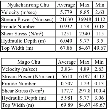
As the stream power for GLOF is more as compare to 50 and 100 year flood, it can be concluded that along with water high sediment laden debris will flow to the downstream project sites. Because of the valley characteristics and variations of the cross sectional areas, the velocity profile shows wide range of variations. The range for hydraulic parameters in the catchments of Nyukcharong Chu and Mago Chu are presented in Table 3.
Nyukchanrong Chu Average Max Min Velocity (m/sec) 5.779 8.85 2.63 Stream Power (N/m.sec) 21630 36948 4112 Froude Number 0.932 1.58 0.18
Table 3. Range of hydraulic parameters along the river reaches of Mago Chu and Nyukcharong Chu
4. CONCLUSION
In this present study, the following conclusions are drawn from analysis of satellite imagery, topographic data, flow data and GLOF simulation at major potential HEP in Tawang Basin.
4.1 Identification and Mapping of Potential Glacial Lakes in Tawang Basin
Multispectral and multi date satellite imagery from Landsat-8 were used to identify glacial lakes in the inaccessible region in Tawang Basin. An algorithm along with decision format was developed by coupling spectral indices, topographic data and spatial information from Google Earth for high altitude lakes in the basin. In both Nyukcharong Chu and Mago Chu catchments, a total of 37 lakes, those are having area more than 0.1 km2 were identified using multi-date and multispectral remote sensing data and the manual digitization of lake was done. The biggest Lake in the catchment area has a surface area of 22.6 km2. This lake is the origin of Nyukcharong Chu stream. For the criticality assessment of GLOF producing lakes, the critical parameters such as stream order, area, proximity, slope and elevation have
been used. Out of the 37 lakes, 2 lakes, (Lake ID-20) is in Mago Chu catchment and other one (Lake ID-7) in Nyukcharong Chu catchment were categorized as medium vulnerable lakes and considered for further GLOF simulation.
4.2 GLOF Simulation
GLOF hydrograph obtained is a function of volume of water that the lake hold and the full formation time for breach development. Hydrodynamic modelling provides reasonable estimates of the GLOF at the downstream HEP sites and the details of the attenuated flood peaks at different locations and their arrival timing. Peak discharge obtained from Lake ID-20 of Mago Chu catchment was attenuated at Mago Chu HEP site, with an arrival timing of 2 hour and from Lake ID-7 to Nyukcharong Chu Barrage site, with an arrival timing of 1 hour and 10 min.
4.3 GLOF Impact on HEP Site
Instead of adopting conventional reservoir based hydropower projects, a run-of-river environmental friendly project needs to be employed for reducing the impact of GLOFs. Machine operated gated structures, that to be regularly operated, in the (half an hour basic) should be planned. Gated structures with little ponding will also be a good substitute of traditional Hydro dams. In such scheme, the normal course of the river will remain un-altered. Run-of-River project should put debris removal structures.
REFERENCES
Bajracharya, B., Shrestha, A.B., Rajbhandari, L., 2007. Glacial Lake Outburst Floods in the Sangarmatha Region. International Mountain Society, Vol.27 (4), pp. 336-344.
Bolch, T., Kamp, U., 2006. Glacier Mapping in High Mountains Using DEM's, Landsat and ASTER Data. Proceeding of 8th International symposium on High Mountain Remote Sensing Cartography.
Bolch, T., Peters, J., Yegorov, A., Pradhan, B., Buchroither, M., Balagoveshcensky, V., 2011. Identification of potentially dangerous glacial lakes in the northern Tien Shan Springer Science +Business Media B.V.,Net Hazards, 59 pp. 1691-1714.
Claguea. J., Evans.S.G., 2000. A review of catastrophic drainage of moraine-dammed lakes in British Columbia. Quat. Sci. Rev. 19, pp. 1763-1783.
Dahms S. H., 2006. Moraine dam failures and glacial lake outburst floods.
Huggel C, kaab A, Haeberli W., Teysseire P, Paul F., 2002. Remote sening based assessment of hazards from glacier lake outburst: a case study in the Swiss Apls. Can Geotech J, 39(2), pp. 316-30.
Huggel, C; Haeberli, W; Kääb, A; Bieri, D; Richardson, S., 2004. An assessment procedure for glacial hazards in the Swiss Alps. Canadian Geotechnical Journal. 41, pp. 1068-1083.
Jain, Sanjay K., Lohani, Anil K., Singh, R.D., Chaudhary, A., Thakural, L.N., 2012. Glacial lakes and glacial lake outburst flood in a Himalayan basin using remote sensing and GIS. Springer Science +Business Media B.V., Net Hazards 62, pp. 887-899.
Mool. P. K., Shrestha. A. B., 2011. Glacial lakes and glacial lake outburst floods in Nepal International Centre for Integrated Mountain Development GPO Box 3226, Kathmandu, Nepal. Vol 978(92), pp. 1936-1943.
Reynolds J. M., 2006. Role of geophysics in glacial hazard assessment. First break volume 24.
Shrestha, A.B., Eriksson, M., Mool, P., Ghimire, P., Mishra, B., Khanal, N.R., 2010. Glacial lake outburst flood risk assessment of Sun Koshi basin, Nepal" Geomatics, Natural Hazards and Risk, vol 1 (2), pp. 157-169.