isprsarchives XXXIX B3 29 2012

A NEW APPROACH OF DIGITAL BRIDGE SURFACE MODEL GENERATION

Hui Ju

Department of Civil, Environmental and Geodetic Engineering, The Ohio State University,

470 Hitchcock Hall, 2070 Neil Avenue, Columbus, OH 43210, USA – ju.32@osu.edu

Commission III, WG III/1

KEY WORDS: LiDAR Intensity Image, Aerial Image, Co-registration, DTM/DSM, Digital Bridge Surface Model

ABSTRACT:

Bridge areas present difficulties for orthophotos generation and to avoid “collapsed” bridges in the orthoimage, operator assistance is required to create the precise DBM (Digital Bridge Model), which is, subsequently, used for the orthoimage generation. In this paper, a new approach of DBM generation, based on fusing LiDAR (Light Detection And Ranging) data and aerial imagery, is proposed. The no precise exterior orientation of the aerial image is required for the DBM generation. First, a coarse DBM is produced from LiDAR data. Then, a robust co-registration between LiDAR intensity and aerial image using the orientation constraint is performed. The from-coarse-to-fine hybrid co-registration approach includes LPFFT (Log-Polar Fast Fourier Transform), Harris Corners, PDF (Probability Density Function) feature descriptor mean-shift matching, and RANSAC (RANdom Sample Consensus) as main components. After that, bridge ROI (Region Of Interest) from LiDAR data domain is projected to the aerial image domain as the ROI in the aerial image. Hough transform linear features are extracted in the aerial image ROI. For the straight bridge, the 1st order polynomial function is used; whereas, for the curved bridge, 2nd order polynomial function is used to fit those endpoints of Hough linear features. The last step is the transformation of the smooth bridge boundaries from aerial image back to LiDAR data domain and merge them with the coarse DBM. Based on our experiments, this new approach is capable of providing precise DBM which can be further merged with DTM (Digital Terrain Model) derived from LiDAR data to obtain the precise DSM (Digital Surface Model). Such a precise DSM can be used to improve the orthophoto product quality.

1. INTRODUCTION

Nowadays, more and more orthophotos of highway corridor areas are demanded for the purpose of maintaining and advancing the public transportation system. Nevertheless, bridge areas present challenges, as without operator assistance, distortion is usually introduced. In order to avoid “collapsed” bridges in the orthoimage, a precise DBM (Digital Bridge Model) is needed. The work presented in this paper is focused on a new method to generate the precise DBM based on fusing LiDAR data and aerial imagery. Actually, fusing LiDAR data and aerial imagery to create the precise digital man-made object model has been widely investigated in the photogrammetric community. However, most methodologies utilize LiDAR elevation information only; the LiDAR intensity information is mostly ignored. The main difference with other methods is that our method is based on the co-registration between the LiDAR intensity and aerial image pair.

1.1 Literature Review

Although LiDAR data can directly provide accurate and dense surface measurements, it cannot well determine the man-made object boundaries due to the irregular and sparse nature of LiDAR points at break lines. On the other hand, the man-made object boundaries can be well extracted from aerial imagery. Fusing clean and smooth boundaries from aerial imagery and LiDAR elevation data becomes an efficient way to create the digital man-made object model (Kim et al., 2008; Rottensteiner and Briese, 2002; Sampath and Shan, 2007; Vosselman, 1999). Reviewing related publications, most of the research is focused on precise digital building modelling. The main idea is to extract 2D outlines of buildings from aerial images, then project them to the 3D LiDAR data space via the colinearity equation,

and subsequently, compare them with 3D linear features extracted from LiDAR data to obtain the smooth and precise digital building models. Those methods show good results for automated generation of polyhedral building models for complex structures (Kim and Habib, 2009; Wu et al., 2011); however, implementation of these methods could be complex and the computation load could be heavy. Most earlier research is focused on either generating DBM (Digital Bridge Model) based on analysis of LiDAR point cloud profile (Sithole and Vosselman, 2006) or bridge boundary extraction from DTM (Geopfert and Rottensteiner, 2010). Nevertheless, the determination of man-made object boundaries in LiDAR data is rather complex. If the co-registration between LiDAR intensity and other high resolution imagery can be established, it is not necessary to generate the perfect DBM from LiDAR data domain, as the LiDAR data derived coarse DBM can be refined by introducing smooth bridge boundaries, extracted from the high resolution image. This is the concept of the proposed approach.

1.2 Proposed Method

In this paper, the man-made objects to be modelled are bridges whose shape is either straight or curved. The new idea is to transfer smooth bridge boundaries extracted from the aerial image to the LiDAR intensity image via the co-registration between them. Ultimately, the accurate DBM is finalized in the LiDAR data domain by fitting smooth boundaries to the coarse boundaries derived from LiDAR data. The co-registration method was firstly proposed based on our earlier research work of co-registration between satellite and LiDAR intensity images (Toth et al., 2011).

In the following sections, first, the bridge data used for testing is described. Then, the entire workflow of DBM generation based on straight and curved bridge shapes is presented and explained step by step. The last section provides results and discussion.

2. TEST DATA

For this study, high resolution DMC aerial images and LiDAR data of highway 161 corridor area in Franklin County, Ohio, USA were provided by ODOT (The Ohio Department of Transportation), shown in Figure 1. A straight bridge enclosed in a black rectangle ROI (Region Of Interest) and a curved bridge enclosed in a red rectangle ROI are selected as test bridges.

Figure 1. Straight test bridge (1) and curved test bridge (2)

Using the aerial image footprint, LiDAR intensity image is generated from LiDAR data; the image resolution is set to 1m GSD (Ground Sample Distance). Figure 2 show the aerial image (a) and its corresponding LiDAR intensity image (b).

(a) (b)

Figure 2. Aerial image (a) and LiDAR intensity image (b)

3. METHODOLOGY

The proposed workflow consists of four steps: derivation of coarse DBM from LiDAR data, co-registration between aerial and LiDAR intensity image pair, extraction of smooth boundaries from aerial image and precise DBM generation.

3.1 Coarse DBM Generation

For our tests, the bridge ROI is manually selected in the LiDAR intensity image which is a rasterized LiDAR point cloud, created by using the highest intensity value of points falling in a ground cell. 1m sample size is used to generate the LiDAR intensity image. The relation between LiDAR intensity image space and LiDAR data mapping system is the following 2D transformation:

� − �0=� − �_���0

� − �0=� − �_���0

(1)

where (x, y) is the image coordinate and (E, N) is the corresponding LiDAR mapping Easting and Northing coordinate

(x0, y0) is the image coordinate system origin, which is defined as the upper left corner, (E0, N0) is the corresponding LiDAR mapping Easting and Northing coordinate

Once GSD is fixed, the bridge ROI in the LiDAR intensity image can be easily transformed to ROI in the LiDAR data domain, which is the 3D LiDAR ROI point cloud used to generate the coarse DBM.

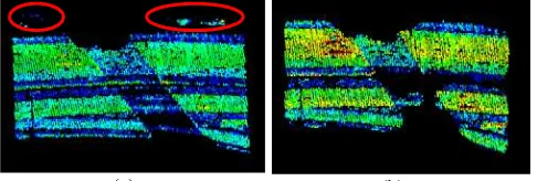
First, ground points and non-bridge points should be filtered out. Ground points can be easily removed based on elevation analysis. For non-bridge points having similar height as the bridge surface, the intensity data can be used for filtering. Nevertheless, pavement markings and/or vehicles on the bridge may have different reflectance characteristics, and thus, those points can be also removed which could create void areas in the bridge surface. In addition, outlier points may also exist; see the isolated point clusters in red ellipses in the Figure 3 (a). In order to trim those sparse outlier points, a statistical outlier removal filter based on statistical analysis on each point’s neighbourhood is also applied to clean the bridge points. For each point, the 2D mean distance from it to its closest n points is computed. It is assumed that those mean distances obey a Gaussian distribution. Then, points with mean distances outside the interval, defined by the global distances mean and standard deviation, can be regarded as outliers and removed from the bridge points; see differences between Figure 3 (a) and (b).

(a) (b)

Figure 3. Elevation/intensity filtered bridge surface (a) and cleaned by a statistical filter (b)

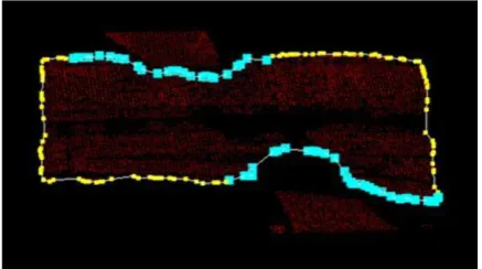
3D RANSAC (Fischler and Bolles, 1981) plane estimation is applied on those cleaned bridge points to find the robust 3D plane parameters. Elevation of bridge points is recomputed through the 3D plane equation using the estimated 3D plane parameters. The newly computed points should be perfectly on the bridge surface defined by the estimated plane. Subsequently, concave hull boundary estimation is performed on the refined bridge surface points, as the bridge surface has a concave shape. In addition, points on bridge boundaries are also determined

based on checking elevation value with respect to their neighbourhood in a circular searching area, since the elevation difference should be large for boundary points and small for non-boundary points. The concave hull polygon (white) connecting those concave hull boundary points (yellow) and the bridge boundary points (blue) are illustrated in the Figure 4.

3.2 Co-registration

In our earlier research on multiple-domain imagery co-registration, a new approach based on LPFFT (Reddy and Chatterji, 1996; Wolberg and Zokai, 2000), Harris Corners, PDF mean-shift matching (Comaniciu et al., 2003) and RANSAC (Fischler and Bolles, 1981) affine transformation estimation was proposed (Toth, et al., 2011). With a limited dataset, the proposed method achieved promising results, and thus, it is applied to estimate the geometric transformation which is assumed an affine transformation, between the LiDAR intensity and aerial images. Figure 5 shows the workflow of the proposed co-registration approach.

Figure 4. Concave hull boundary points (yellow) and bridge boundary points (blue)

Figure 5. Workflow of the affine transformation estimation

First, the similarity transformation regarded as the coarse geometric transformation is estimated via a standard LPFFT registration method. Next is the similarity validation step where the scale and rotation parameter are validated based on a Monte Carlo process; more precisely, a Monte Carlo test is performed for a set of scale and rotation values computed from the originally estimated parameters (�₀,�₀) via following equations:

� ≔{�|�_�=�₀±� ⋅ ��}

� ≔{�|�_�=�₀±� ⋅ ��} (2)

The second image is transformed using each scale and rotation combination in the set. If the estimated scale and rotation parameters are correct, the images should have comparable orientation and scale. Then, FFT-accelerated NCC (Normalized Cross Correlation), an efficient NCC computation method, can be used to estimate the translation parameters for each image pair by searching the maximum NCC values. Those maximum NCC values of all image pairs should be kept at a significantly

high level, which means small scale and rotation changes around the correct scale and rotation still lead to a high NCC value. If the estimated scale and rotation are wrong, the maximum NCC values of all image pairs should be small. Figure 6 (a) shows the typical NCC surface based on the wrong

(�0,�0) and (b) based on the correct (�0,�0) paramters. If the

EOPs (Exterior Orientation Parameters) of aerial image are available, it is also possible to introduce a rotation angle constraint to improve the performance of similarity transformation estimation. According to our experiences, the scale and rotation parameters can be reliably estimated based on orientation angle constraint and the Monte Carlo validation. The translation parameters, however, may not be easily estimated by LPFFT. Therefore, translation parameters are estimated through the edge NCC matching method.

(a) (b) Figure 6. NCC value surface; wrong scale and rotation parameter (a) and correct scale and rotation parameter (b)

The second image is transformed using the estimated scale and rotation angle, so the image pair should have similar orientation and scale. A number of rectangle reference patches are generated in the first image, and subsequently, those reference patches are matched in the second image. Thus, the translation parameters can be computed as the center point image coordinate differences between the reference patch and matched patch. The correct translation is determined by a statistical analysis of all computed translations. The translations with highest frequency are accepted as correct translations, see Figure 7.

(a) (b) Figure 7. NCC value surface; wrong scale and rotation parameter (a) and correct scale and rotation parameter (b)

The Harris Corners detector is used to extract feature points, and circular regions cantered on strong HC features are created in both images, including the imported locations from the other image. Next the scale- and rotation-invariant PDF descriptor is used to describe the circular feature region. The PDF function is represented in a 256-dimensional feature descriptor. The similarity between two feature descriptors is computed via the Bhattacharyya Coefficient, which is the cosine of angle correlation between the two feature descriptors, defined as:

�=�(�,�) =� ��_�⋅ �_�=���� ≥0 �

�=1

(3)

where _∑�_{�=1���= ∑}�_{�=1���}=1

The maximum similarity score ρ is 1, which means the two feature descriptors are exactly the same. The minimum similarity score is 0 which means the two feature descriptors are orthogonal to each other; in other words, they don’t have any relation. PDF matching is implemented based on mean-shift searching strategy. Finally, affine transformation parameters are estimated based on the PDF-matched tie points. Note that RANSAC is used to remove the blunders. Figure 8 illustrates the co-registration results after RANSAC blunder detection; the RANSAC threshold value is set to 0.5-pixel.

Figure 8. Co-registration result

3.3 Extracting Smooth Bridge Boundaries in Aerial Image

Hough linear transform is applied to the bridge ROI in the aerial image to extract the bridge boundaries. For each Hough transform identified linear feature, its Hough transform angle is also recorded, which can be used to determine the bridge direction and remove the non-bridge linear features. For a long curved bridge, Hough circle transform was attempted to extract the curved boundaries; nevertheless, the performance was not stable. Alternatively, short linear features are extracted along the curved bridge boundaries. Since Hough linear transform cannot be directly used to extract long curved bridge boundaries, the long curved bridge ROI is divided into several small sub-ROIs, as shown in Figure 9.

(a) (b)

Figure 9. Sub-ROIs of a curved bridge ROI (a) and short linear features in sub-ROI 4 (b)

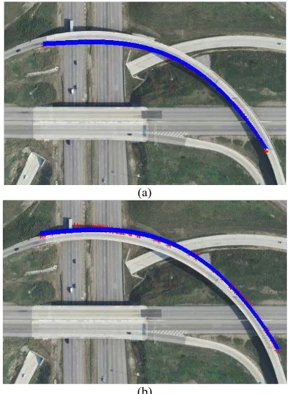
Then, it is possible to obtain short linear features in each sub-ROI. Hough linear features in all sub-ROIs are merged together to form the complete Hough transform linear features along the long curved bridge boundaries. The endpoints of linear features are used to generate the smooth bridge boundary, see red points in Figure 10.

It is also necessary to determine points of upper and lower boundaries for the smooth boundary generation. In order to simply separate the upper and lower boundary, all linear features are rotated to align to the horizontal direction based on the recorded Hough transform angles. This step is performed in each sub-ROI for the curved bridge. If the bridge is rotated to horizontal direction, upper and lower boundaries can be separated based on comparing the Y coordinate. For straight bridge boundary, 1st order polynomial function is used to fitting those boundary points; for curved bridge boundary, 2nd order polynomial function is used. Once the polynomial function parameters are estimated, the smooth boundary can be then represented in the dense sample points computed via the polynomial function, see blue points in Figure 10.

(a)

(b)

Figure 10. Smooth boundary points computed via 2nd order polynomial function (blue) according to the Hough linear

feature endpoints (red)

3.4 Precise DBM Generation

If the affine transformation between LiDAR intensity and aerial image is established, smooth boundaries can be transformed from the aerial image to the LiDAR intensity image as well as to the LiDAR elevation data. The upper and lower boundaries are shifted to best fit the upper and lower coarse boundary from the coarse DBM. Figure 11 shows the smooth boundaries, fitting the coarse boundaries. The void area between the smooth boundary (pink) and the coarse boundary (blue) extracted from LiDAR data should be filled in to form a precise DBM. In addition, the elevation values of the smooth boundary points are computed based on interpolating its neighbour points’ elevation values. The precise DBM can be merged with the DTM derived from LiDAR data to form a precise DSM.

(a)

(b)

Figure 11. Smooth boundary points computed via 2nd order polynomial function (blue) according to the Hough linear

feature endpoints (red)

4. RESULTS AND CONCULUSION

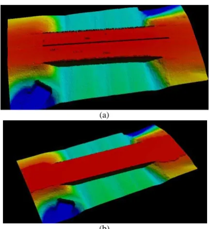
A comparison between bridge ROI DSM derived from LiDAR data and DSM based on the precise DBM is given in Figure 12 and Figure 13 for the test bridge 1and 2, respectively.

(a)

(b)

Figure 12. Bridge ROI DSM derived from LiDAR data (a) and DSM based on the precise DBM (b) (bridge 1)

(a)

(b)

Figure 13. Bridge ROI DSM derived from LiDAR data (a) and DSM based on the precise DBM (b) (bridge 2)

Clearly, the bridge ROI DSM is refined in both cases; the surface and outlines of the bridges are smoother. For the test bridge 2, the “collapsed” bridge section due to tree crowns is well repaired. DSM with precise DBM can be used to improve the orthophoto generation of the highway corridor areas. In this paper, a new precise DBM generation method based on fusing LiDAR and aerial image data is introduced. The novel idea is to transfer smooth bridge boundaries extracted from the aerial image to the LiDAR data via the established co-registration between LiDAR intensity and aerial images. Note only approximate exterior orientation of the aerial image should be known. In case aerial imagery is not available, other high resolution satellite image can be also used. In this paper, the method is applied to produce precise DBM of straight and curved bridges by fusing LiDAR data and aerial images. In future research, complex multiple-layer bridge models using this methodology will be investigated. In addition, the possibility to apply this method to generate digital building model of complex building structures will be also explored.

REFERENCE

Comaniciu, D., Ramesh, V., Meer, P., 2003. Kernel-based object tracking. IEEE Transcations on Pattern Analysis and Machine Intelligence, Vol. 25, Issue 5, pp. 546-577

Fischler, M. A., Bolles, R. C., 1981. Random sample consensus: a paradigm for model fitting with applications to image analysis and automated catography. Communications of ACM, Vol. 24, pp. 381-395

Goepfert, J., Rottensteiner, F., 2010. Using building and bridge information for adapting roads to ALS data by means of network snakes. International Archives of Photogrammetry,

Remote Sensing and Spatial Information Sciences, Vol. 38, Part 3A, pp. 163-168

Kim, C., Habib, A., 2009. Object-Based Integration of photogrammetric and LiDAR data for automated generation of complex polyhedral building models. SENSORS, Vol. 9, Issue 7, pp. 5679-5701

Kim, C., Habib, A., Chang, Y., 2008. Automatic generation of digital building models for complex structures from LiDAR data. In: The International Archives of Photogrammetry and Remote Sensing, Vol. 37, pp. 456-462

Reddy, B. S., Chatterji, B. N., 1996. An FFT-based technique for translation, rotation and scale-invariant image registration. IEEE Transactions on Image Processing, Vol. 5, Issue 8, pp. 1266-1271

Rottensteiner, F., Briese, C., 2002. A new method for building extraction in urban aeras from high-resolution LiDAR data. In: The International Archives of Photogrammetry and Remote Sensing, Vol. 34, pp. 295-301

Sampath, A., Shan, J., 2007. Building boundary tracing and regularization from airborne LiDAR point clouds. Photogrammetric Engineering and Remote Sensing, Issue 73, 805-812

Sithole, G., Vosselman, G., 2006. Bridge detection in airborne laser scanner data. ISPRS Journal of Photogrammetry and Remote Sensing, Vol. 61, Issue 1, pp. 33-46

Toth, C., Ju, H., Grejner-Brzezinksa, D., 2011. Matching between different image domains. In: Lecture Notes in Computer Science, PIA 2011, Munich, Germany, Vol. 6952, pp. 37-47

Vosselman, G., 1999. Building reconstruction using planar faces in very high density height data. In: The International Archives of Photogrammetry and Remote Sensing, Vol. 32, 87-92

Wolberg, G., Zokai, S., 2000. Robust image registration using Log-Polar transform. In: International Conference on Image Processing Proceedings, Vol. 1, pp. 493-496

Wu, J., Jie, S., Yao, W., Stilla, U., 2011. Building boundary improvement for true orthophoto generation by fusing airborne LiDAR data. In: 2011 Joint Urban Remote Sensing Event, Munich, Germany, pp. 125-128

ACKNOWLEGEMENT

The aerial imagery and LiDAR data provided by ODOT (Ohio Department of Transportation) for this study is greatly appreciated.