Phase Diagram, Density, And Current Density Profiles Of Totally
Asymmetric Simple Exclusion Process For A Junction With Two Entrances
and Two Exits
M. Za’im
1and W. S. B. Dwandaru
21
Sekolah Pascasarjana, Gadjah Mada University, Bulaksumur,
Yogyakarta, 55281, Indonesia
2
Physics Education Department, Yogyakarta State University, Karangmalang, Yogyakarta,
55281, Indonesia
E-mail: [email protected]
1, [email protected]
2Abstract
A dynamical model called the totally asymmetric simple exclusion process (TASEP) in one dimension (1D) is a widely-held particle hopping model which has developed into a reference model for studying non-equilibrium driven systems in particular transport phenomena. In this study, the TASEP is extended for a case of a junction with two entrances and two exits. The model is specified by a dynamical rule and boundary conditions. The dynamical rule determines the movement of particles and in this case the sequential updating dynamics is applied. The boundary condition used is the open boundary conditions, where particles may enter or exit the lattice sites. The density of the TASEP is governed by a continuity equation, which is solved numerically, such that a phase diagram and the current density profiles are obtained. The result shows that there are ten density phases produced, viz.: low density, high density, coexistence phase, maximal current, low density-low density, high density-high density, high density-maximal current, low density-maximal current, maximal current-high density, and maximal current-low density. The current density is generally constant throughout the lattice sites, except at the junction where a spike occurs.
Keywords: current density profile, density profile, open boundary condition, phase diagram, sequential updating dynamics.
I.
Introduction
The totally asymmetric simple exclusion process (TASEP) in one dimension (1D) is a standard mathematical model to investigate a wide range of non-equilibrium phenomena in physical sciences, including physics, chemistry, and biology (Chowdhury, 2003; Hinsch et.al., 2006; Shaw et.al., 2003). In general, the TASEP is a particle hopping model whereby hard core particles occupying one-dimension discrete lattice sites may jump to their right nearest neighbour sites provided that there are no particles occupying the right neighbour sites. The jump may occur in one direction only, in this case, to the right. Originally, the TASEP is used to study the kinematics of polymerization (Pipkin and Gibbs, 1966; Simha and Zimmerman, 1963), e.g. for DNA and RNA synthesis on DNA templates (MacDonald et.al, 1968). Since then the model has been used to investigate one dimensional transport systems (Hinsch et.al., 2006; Chowdhury et.al., 2005; Hinsch and Frey, 2006). Variation to the TASEP has been conducted by Parmeggiani et.al. (2004) by coupling
it to Langmuir kinetics. This produces a domain wall and rich phase diagram.
site with rate k given that there is no particle occupying the right nearest neighbour site (MacDonald et.al., 1968).
The density profiles of the TASEP are described by a phase diagram. The phase diagram for the TASEP in 1D with sequential updating and open boundary conditions is based upon on the horizontal-axis and on the vertical-axis (shown in Picture 1). and β may take the numerical values with sequential up-dating and open boundary conditions. The horizontal axis is the constant input rate, , and the vertical axis is the output rate, . The equation shown is the current density of each of the phase. There four phases illustrated, i.e.: low density, high density, maximal current, and coexistence phase.
Here, the objective of this research is to extend the well-known TASEP in one dimension into a less-known, but potentially important model that is the TASEP with a junction. By extending the lattice sites into a junction, the hopping of particles may be varied not just to the right nearest neighbour sites, but also to the upper nearest neighbour sites. Foster et.al. (1994) has studied the stationary states of a two dimensional lattice gas model with exclusion which consists of two species. Furthermore, an extensive Monte Carlo simulation has been done by Pronina
et.al. (2004) in order to study the two-channel totally asymmetric simple exclusion process. However, to the best of our knowledge, the numerical study of the TASEP for a case of a junction with two entrances and two exits has not been done before.
In this case, a special arrangement of the TASEP is put forward, i.e. joining two TASEPs in 1D at the centre of each TASEP perpendicular to each other (Picture 2). Hence, the phase diagram and the current density profiles of the TASEP with a junction may be discussed based on the same respective quantities of the TASEP in 1D. For this case, the TASEP in 1D with input and output rates,
1 and 1, respectively, is placed horizontally (path i.e.: N = 101. However, the joining of both paths at the centre resulted in the total number of particles of 201 lattice sites.
sites ([N+1]/2,1) to sites ([N+1]/2,N–1), which is ku = 0.5. A particle may enter site (1,[N+1]/2) or site ([N+1]/2,1) and exit site (N,[N+1]/2) or site ([N+1]/2,N) with rates 1, 2, 1, 2, respectively.
Hence, the junction has two entrances and two exits.
Picture 2: TASEP in 2D for a junction with two entrances and two exits.
There are two primary physical quantities that are discussed in this research that is i) density and ii) current density. The density [i(t)] is the average ensemble of particles in occupying a lattice site-i at time t. Meanwhile, the current density [Ji(i+1)(t)] is
the average number of hopping conducted by particles from site-i to site-(i+1) at time t. The relationship between the density and the current density is given by a continuity equation, viz.:
.t t
i i
i
J 1
(3)
As the lattice sites are discrete, a simple Euler method may be used to modify the left hand side of Eq. (3), that is Ji(t) = Ji(i+1)(t) – J(i-1)i(t), such that
the formal solution of Eq. (3) can be written as,
'
'
'
.t
i i i
i i
i t t dt J t J t
0
1 1
1
(4)
The left hand side of Eq. (4) is obtained by modifying the right hand side of Eq. (3) considering discrete time steps, such that i(t)/t i(t+1) -
i(t). Furthermore, the current density of the TASEP
in 2D can be written as (Dwandaru, 2010):
i eˆ
ii ˆe
i
i eˆ
,i t k t t t
Jr x r x 1 x (5)
and
i ˆe
i
i eˆ
i
i eˆ
,i t k t t t
Juy u y 1 y (6)
where Eq. (5) and Eq. (6) are the current densities of particles moving from site- to site-(i+êx) and site- to site-(i+êy), respectively. The equations are
obtained via a relationship between the hard core lattice gas model and the TASEP extended to two dimensions (Dwandaru and Schmidt, 2007). The hard core lattice gas model is studied using density functional theory (DFT) which is extended to lattice systems via the lattice fundamental measure theory (LFMT) (Lafuente and Cuesta, 2002; Lafuente and Cuesta, 2004). There are three relationship put forward based upon (Dwandaru, 2007), that is, (i) the particle of the TASEP is associated to the hard core particle in the lattice gas that excludes its own site, (ii) the jump of the particle of the TASEP to the right nearest neighbour site is associated to the hard core particle in the lattice gas that excludes its own and its right nearest neighbour site, and (iii) the jump of the particle of the TASEP to the upper nearest neighbour site is associated to the hard core particle in the lattice gas that excludes its own and its upper nearest neighbour site. Hence, the TASEP may be studied using the lattice gas model that consists of three species of particles. This yields three Euler-Lagrange equations of the species of particles via a variational principle. Finally, the density and current densities of the particles in the TASEP are obtained via a linearization of the aforementioned Euler-Lagrange equations.
The evolution of the density with respect to time for the TASEP in 2D may be calculated by inserting eqns. (5) and (6) into (3). This is the main partial differential equation which will be solved. The equation depends on the boundary conditions specified. Hence, the input and output rates determine the density and current density profiles of the TASEP through Eqns. (5) and (6).
II.
Research Method
2.1 Research Variables
Various parameters are used in this study. The parameters are described as follows: i) the input rates of particles from the reservoirs to the lattice system, that is 1 and 2, and ii) the output rates of
particles from site-i to site-i+1 to the right nearest neighbour, kr, i.e.: 0.5, and iv) the hopping rate of particles from site-i to site-i+1 to the upper nearest neighbour site, ku, i.e. 0.5. The independent variable utilized in this research is the time evolution, t, of 5× 10⁵ time steps., and the total number of lattice sites,
which is 201.Finally, the density of particles, , and the current density, j, are functions of time t.
2.2 Research Design
In order to study the density and current density of the TASEP with a junction, the Dev C++ language program is applied, that is by constructing a computer code based on the parameters given above. This is done by providing a set of trial density profile into the right hand side of Eq. (4). Then calculation is made on the right hand side of Eq. (4) such that a new density profile is obtained. The new density profile is inserted to the right hand side of Eq. (4) and a calculation is made, such that another density profile is obtained, and so forth. This iteration procedure is terminated after the density profile converges to its true values or the system reaches a non-equilibrium steady state. Furthermore, by varying the input and output rates, 1, 2, 1, 2,
respectively, the numerical values of the density and current density profiles are obtained. To observe the density and current density profiles, graphs of the density and current density as a function of the lattice sites are produced. Finally, the density phases can be determined based on the graphs and shown in a diagrammatic form.
III.
Results and Discussion
3.1 The Phase Diagram of the TASEP in 2D for a Junction with Two Entrances and Two Exits
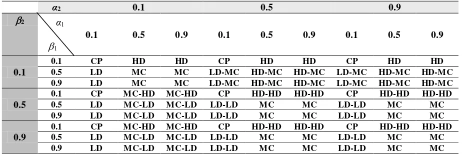
The four way lane TASEP in 2D with two input and two output rates produces eight (8) variants of density phases, i.e.: low density (LD), high density (HD), coexistence phase (CP), maximal current (MC), low density-low density (LD-LD), high high density (HD-HD), high maximal current (HD-MC), and low density-maximal current (LD-MC). It may be noticed that there are four additional combinations of density phases besides the original phases obtained from the TASEP in 1D with open boundary conditions. These phases are LD-LD, HD-HD, LD-MC, and HD-MC. The aforementioned phases are obviously the result of the junction occurring in the lattice system. Table 1 is the phase diagram of the particle density of path 2 and path 1 (see Picture 2), i.e.: (2,2) and
(1,1), respectively. The criteria for obtaining
each of the density phase in Table 1 follows from the density phases of the TASEP in 1D. The LD (HD) phase is obtained if the value of the density is less (more) than 0.5 throughout the bulk. The MC phase is obtained if the value of the density is 0.5 around the bulk. Finally, the CP is gained if there is a shock (domain wall) in the density profile such that LD and HD coexist.
Table 1: The density phase diagram of path 1 and path 2, i.e.: (1, 1) and (2, 2), respectively, for the
four way lane TASEP in 2D with a junction.
α2 0.1 0.5 0.9
2 α1
1
0.1 0.5 0.9 0.1 0.5 0.9 0.1 0.5 0.9
0.1
0.1 CP HD HD CP HD HD CP HD HD
0.5 LD MC MC LD-MC HD-MC HD-MC LD-MC HD-MC HD-MC 0.9 LD MC MC LD-MC HD-MC HD-MC LD-MC HD-MC HD-MC
0.5
0.1 CP MC-HD MC-HD CP HD-HD HD-HD CP HD-HD HD-HD 0.5 LD MC-LD MC-LD LD-LD MC MC LD-LD MC MC 0.9 LD MC-LD MC-LD LD-LD MC MC LD-LD MC MC
0.9
As mentioned before, the phase diagram of the TASEP with a junction and two input and output rates is similar to that of the ordinary TASEP in 1D with open boundary conditions. The main phases of the TASEP in 1D still persist, that is LD, HD, CP,
and MC. However, an additional lane produces a combination of phases, which are LD-LD, HD-HD, LD-MC, and HD-MC.
(i) (ii)
(iii) (iv)
(v) (vi)
Picture 3:The density profiles of the TASEP in 2D for a junction with various input and output rates which are combinationsof density profiles of the TASEP in 1D. The solid (blue) lines are the density profiles of path 1, whereas the dashed (red) lines are the density profile of path 2. In accordance with Table 1, profiles (i), (ii), (iii), (iv), (v), and (vi) show the LD-LD, HD-HD, LD-MC, MC-HD, MC-LD, and HD-MC phases of the density profiles of path 1, respectively.
Take for example 2 = 2 = 1.0. Now, for the
TASEP in 1D with open boundary conditions this would produce a CP where high and low densities
co-exist. However, when another lattice system is embedded in the middle and perpendicular to the previous one, then the density of the system varies with the input and output rates of the latter lattice
dens
it
y
system. It may be observed on the upper-left corner of Table 1, as 1 and 1 get larger, that the phases of
the system may be in LD, HD, or MC. Another case is 2 = 0.1 and 2 = 0.5. Normally, for the TASEP in
1D this case produces a simple LD phase. However, the presence of the junction enriches the phases as increase of 1, which makes the particles possibly go
out from the last site of path 1, making some part of path 2 fall from HD into LD. An example of the HD phase in the TASEP in 1D is when 2 = 0.9 and 2 =
0.1. Adding another path 1 onto path 2 results in a change of the density phase. For 1 = 0.1 and 1 =
0.5 or 0.9, the phase of the system becomes LD-MC. Although there are many particles on path 2, resulted from the high 2 and the low 2, the addition of path
1 makes half of the lattice sites on path 2 become LD and the rest of the lattice sites becomes MC. This means that the HD phase of path 2 may be relieved to a combination of LD and MC phase by adding another path on path 2. This is actually useful in the vehicular traffic phenomena. The last phase of the TASEP in 1D is the MC phase. As an example phase, because of a low density path passing through it, lowers path 2 into a LD-LD phase. Again, this might be useful in the phenomena of vehicular traffic in order to reduce congestion of traffic.
3.2 The Density Profiles of the TASEP for a TASEP in 2D for a junction with two entrances and two exits which resulted from combinations of the density profiles of the TASEP in 1D. In accordance with Table 1, the main density profiles being
discussed are of path 1 (solid blue lines). It may be observed later that the density profiles of path 2 and path 1 are symmetrical, so that just one of the paths may be discussed. Picture 3(i) of path 1 (solid blue line) is the LD-LD phase with 1 = 0.1, 2 = 0.5, 1
= 0.9, and 2 = 0.5. The overall value of the density
profile is lower than 0.5. However, there appears to be a small shock around the middle of the lattice site. This shock is a transition from an LD to another LD. From the beginning of the lattice sites until the middle of the lattice sites the value of the density
overall density profile of the solid blue line is larger than 0.5. From the beginning of the lattice sites, the profile starts from below 0.8, and then becomes flat and constant at 0.8 until the middle of the lattice site. Then an abrupt change to a flat and constant higher density of 0.9 happens until the end of the lattice site. Hence, coexistence between two high density phases happens.
An example of a LD-MC phase is given in Picture 3(iii) for 1 = 0.1, 2 = 0.5, 1 = 0.5, and 2
= 0.1. In this case, the (solid blue line) profile starts from a flat-constant low density of 0.1 until the middle of the lattice site, and then a sudden change occurs to a flat-constant higher value of 0.5 until the end of the lattice site. Thus, coexistence between occurs because of the junction. Furthermore, Picture 3(v) and (vi) look similar to Picture 3(i) and (ii), where the density profiles of path 2 and path 1 are interchanged. This example shows that the density profiles of paths 2 and 1 are symmetric. This is also obvious from the geometric point of view of the lattice system given in Picture 2.
Finally, the current density profiles of the TASEP in 2D with a junction are discussed. The current density determines the average hopping of particles from one site to its nearest neighbour at each time step. As shown above, the profiles which
are being discussed are the current density profiles of path 1 (solid blue lines), i.e. J. These profiles are shown in Picture 4 and are in accordance with the density profiles provided in previous sections.
Picture 4: The current density profiles of the TASEP in 2D for a junction with two entrances and two exits. Picture (i) is the profile of the LD, HD, and CP phases. Pictures (ii), (iii), (iv), (v), and (vi) are the profiles of MC, LD-LD, HD-HD, LD-MC, and HD-MC phases, respectively.
In general it may be observed that the current density profiles are flat throughout the lattice sites, except in the middle of the lattice site where a sharp
spike occurs. This sharp spike indicates that the hopping of particles at the junction is high. The constant values of the current density profiles show
(i)
(iii)
(iv)
(v) (vi)
(ii)
curr
ent
dens
it
y
that the system reaches a non-equilibrium steady state, i.e.: a non-zero but constant current exists in the system. Hence, the applied time evolution of 5 105 time steps is legitimate since using this time
step value, the system may reach a steady state.
IV.
Conclusions
From the results and discussion above, it may be concluded that the density and current density profiles of the TASEP in 2D for a junction with two entrances and two exits depend upon the input (1 maximal current (HD-MC), low density-maximal current (LD-MC), density-maximal current-high density (MC-HD), and maximal current-low density (MC-LD). The first four density phases are equivalent to the density phases of the TASEP in 1D with open boundary conditions, whereas the other six density phases are combinations of the first four. These last six density phases are not found in the TASEP in 1D. The current density profiles are generally non-zero and constant throughout the lattice sites, except at the middle of the lattice site where a sharp peak occurs.
Acknowledgements
M.Z and W.S.B.D would like to thank the Physics Education Department, Faculty of Mathematics and Natural Science, Yogyakarta State University for the support of this research project.
V.
REFERENCES
Chowdury, D., 2003. Traffic Flow of Interacting Self- Driven Particles: RailS and Trails Vehicles and Vesicles, Kanpur: Indian Institute of
Technology,
Hinsch, H., Kouyos, R. & Frey, E., 2006. From Intracellular Traffic to a Novel Class of Driven Lattice Gas Models, Traffic and Granular Flow 2005, Chapter II, Springer, pp. 205 – 222, Shaw, L.B., Zia, R. K. P. & Lee, K. H., 2003. The
Totally Asymmetric Exclusion Process with Extended Objects, a Model for Protein Synthesis, Phys. Rev. E, 68, pp. 021910.
Pipkin, A. C. & Gibbs, J. H., 1966. Kinetics of Synthesis and/or Conformational Changes of
Biological Macromolecules, Biopolymers, 4, 1968. Kinetics of Biopolymerization on Nucleic Acid Templates, Biopolymers, 6, pp. 1-25
Chowdhury, D., Schadschneider, A. & Nishinari, K., 2005. Physics of Transport and Traffic Phenomena in Biology: From Molecular Motors and Cells to Organisms, Phys. Life
Parmeggiani, A, Franosch, T. & Frey, E., 2004. The Totally Asymmetric Simple Exclusion Process with Langmuir Kinetics, Phys. Rev. E, 70, pp. 046101-046121.