Simulation of Land-Use Policies on Spatial Layout with the
CLUE-S Model
Meng Zhang, Junsan Zhao, Lei Yuan
Land Resource Engineering, Kunming University of Science and Technology, Kunming, China.
Email: [email protected]
Keywords: CLUE-S model, land use policies, land use requirements, spatial layout, land use change
ABSTRACT
Currently, the simulation of land use and land cover change is one of the research focuses in land resource management. Models for simulating this topic have been used by lots of scholars. In the process of experiments, especially using the models, to grasp the characteristics of data has a significant impact on the simulation results. With the changes in poli-cies of land use, the spatial layout has shown a new form. How to simulate the change is one of the focuses in the cur-rent Land Resource Management. Therefore, this paper analyzes the curcur-rent land use of the study area in two aspects: the structure and spatial layout, studying on changes in demand according to the current major changes of policies for land use in the area.; based on the in-depth analysis, by making reasonable choices of land use classification and using the logical regression analysis and ROC curve to select driving factor which is suitable for the characteristics of the study area; a reasonable simulation is then conducted for the impact on the spatial layout for land use change policies through CLUE-S model. The result shows that the exact parameters in line with the characteristics of the study area in CLUE-S mode could simulate the land use spatial layout for many land-use policies such as „construction land uphill‟,
„construction land making room for arable land‟, „construction land along the river and road development‟, „key indus-tries land expansion‟. The results have certain significance on land use changes and land use planning. In order to assist the decision making and improve the efficiency of land use, using this method can help the department of land and re-source use to simulate the situation of the land use from the structure and the spatial layout in future according to the demands and the local policies of the land.
1.
Introduction
The simulation of land use cover change is using models and math methods to simulate the changing situations of spatial distribution of land use, which can demonstrate and analyze the spatial variation through the layers and GIS rather than confined to the structured figures for the area, location or related attributes of different land use types.
The Conversion of Land Use and its Effects modeling framework (CLUE) is used to simulate the land use change. Based on it, the CLUE-S is an improved model for small scale regional application, which is more sys-temic, is mainly used to study the rationalization of the land use spatial layout and coordination distribution of the variety demands among the different land use types. Therefore, the CLUE-S model is more applicable to the experimental requirements of this paper.
2.
Introduction of CLUE-S Model
The CLUE-S model is divided into two parts: the de-mand analysis and the dede-mand distribution. statistically, the demand analysis calculates the area changes for all
land use types; while in the demand distribution, area demand for different land types is converted into special land use change in the study area. When all the condi-tions provided, the CLUE-S will compute the most likely changes in land use. In the model, for each raster pixel i, it will calculate the total probability (TPROPi,u)
specif-ic to each land use type u according to the formula:
, ,
i u i u u u
TPROP
P
ELAS
ITER
. (1) where Pi,u is the suitability of land use type u for the location i; the ELASu refers to the conversion elasticity for land use u; ITERu is the iteration variable for land use type u, which marked the relative competitiveness of this type. For all types of land use, when the distribution area is less than the demand area the iteration variable will rise, and when excessive it will down.3.
Analysis of the Regional Situation
3.1.
Overview of the study area
ter-rain. As shown in Figure 2, the terrain of the study area can be divided into three parts: the western, the central and eastern: the western is of high altitude, slope, and vegetation type of forest, with a few garden plot, arid land, irrigated land, villages and natural reserves; the central area is of flat terrain and the most of construction and irrigated land, with towns nearby the highway and the main channel, and irrigated land scattered with vil-lages and other agricultural land; the east area is flat, covered arid land, with the most land of easy grade compared with the western topography.
3.2.
Data and Adjustment of Land Classification
The data is from the second national land survey data-base, base period 2009. There are twenty-three the third level land use types in the study area. The CLUE-S mod-el can only simulates 12 kinds of space layout of land changes at one time, and the classification and setting of different land use types will greatly affect the function of the selected driving factors. Therefore, it is necessary to make pertinent division among the 23 types according to the situation and characteristics in the study area so as to rank the land use types of close spatial relationships, same characteristics or same land use demand into one class for effective simulation. The 23 land use types could be adjusted and re-classified as follows.
Paddy field linking together with the irrigated field, their location and land use requirements are roughly the same. So they are classified into „paddy field and
irrigated land‟.
The pond of agricultural land and facilities scattering in paddy field, irrigated land and arid land could be unified into „other land‟.
The land of small areas for mining, railway, highway, reservoir, hydraulic construction, scenic and special use, rivers and beaches, , with higher requirements on the conditions of land use and thinner probability for transforming into the other land use types. There are no increasing needs of land use for this type, so they are unified into „theother unchanged land‟.
The adjusted spatial distribution map and grid quantity statistics of the 9 land use types are as follows. (1 hectare for 1 gird area) After adjustment, the area of the forest is the largest in the study region, the second is the paddy field and dry land, and the area of other land use type is much less.
4.
Simulation for the change of the land use
4.1.
Analysis on the land use policies
According to the local land use planning of the study area, the development of social economy, the policies
about the land use change and the development prospect of the three major industries, the major policies which affect the land use change from now to 2015 can be summarized as follows.
1) By 2015, the construction land area will increase 34 hectares, the flower planting area will increase 609 tares and the cultivated land area will increase 232 hec-tares in the study region.
2) The land use policy is „developing along river and road‟ for the foreign industry.
3) In the policy of „construction land up the hill (low mound and gentle slope)‟, construction land provides the land for the cultivated land.
4) All of the land use planning must be in accordance with the principles of „centralized layout‟ and „the inten-sive use of land‟.
4.2.
Data preparation
Before using the CLUE-S model to simulate the change of land use, lots of files should be prepared in the instal-lation path of the model. Of all of the files, the text file can be edited directly, while others need preliminary analysis on the layer by the Arc GIS software, then con-verted to raster data and output as ASCⅡ format.
Table1. Summary of the files of the CLUE-S model needed by the experiment
File name Representative meaning File number
cov_all.0 Distribution grid map
con-tains all the land use type 1
cov1_*.0 Distribution grid map
con-tains each land use type 9
region*.fil Raster map of land use
change restricted region 1 or more
demand.in1 The land use demand of
each year 1
allow.txt Change matrix 1
alloc1.reg Logistic regression results 1
main.1 Main parameter file 1
1) Determining the grid size.
Simulation of Land-Use Policies on Spatial Layout with the CLUE-S Model 3
CLUE-S model, the unit shall be in hectares. According to the CLUE-S model application case, using three grid area, 6.25 hectares (i.e. grid size of 250m), 1 hectare (grid size of 100m) and 0.4096 hectares (grid size of 64m) to simulate the change of the land use. And finally, 1 hectare is selected as the experimental grid size, for its computation convenience and moderate gird map display and so will not reduce the speed and the accuracy of the calculation.
2) Preparation for the file of the restricted region. In the file region1.fil (limit change area), with no na-ture reserve in the study area, the land use polygon is zoned for land use change restricted area since it will not change under normal circumstances or occurs only a small change in a particular year, and it will be made mask in order to ensure that the land use polygon under the mask does not participate in the land use change.
3) Preparation for the file of the area demands.
In the file demand.in1, according to the land demand of the land use change of the study area in the simulated year, the area of the garden and the plough land should be increased. In the plough land, the area of the paddy field and irrigated land will increase because of the move of the construction land, and area of the arid land re-mains unchanged. The area of the Village land, the con-struction land and other agricultural land will increase a little. The new construction land will be distributed ac-cording to a certain proportion based on the present area ratio of village land and construction land, the transfer and change characteristics of the village land with the area expansion and position change of the cultivated land and the land use demand of the village land and the con-struction land in the simulated year. The other unchanged land will maintain the original area. The area of forest and natural reserve will reduce.
Table2. Summary of the demands of all the land use types from 2009 to 2015
Unit: the number of the grid
2009 3263 4159 246 1303 5958 579 716 715 532 17471
2010 3302 4159 247 1405 5827 581 720 699 532 17471
2011 3340 4159 249 1506 5695 583 723 683 532 17471
2012 3379 4159 250 1608 5564 585 727 668 532 17471
2013 3418 4159 251 1709 5432 587 731 652 532 17471
2014 3456 4159 252 1811 5301 589 735 636 532 17471
2015 3495 4159 254 1912 5170 591 738 620 532 17471
4) Selection for the driving factors.
In the setting of the file sclgr*.fil (driving factor), ac-cording to the present situation of land use and the land use policies of the study area, different kinds of the land area, location and other factors, 11 driving factors have been selected preliminarily. The 11 driving factors are altitude (S0), distance to the river (S1), distance to the reservoir water and the hydraulic construction land (S2), distance to the arid land (S3), elevation level (S4), dis-tance to the road (S5), disdis-tance to the irrigate land (S6), distance to the garden (S7), distance to the reservoir wa-ter (S8), farmland slope grade (S9) and slope grade (S10). These driving factors should be converted to raster data by Arc GIS software, and then output as ASCⅡ file. By
applying the CLUE-S model with convert.exe software,
different land use type files and different driving factors can be transformed to one file with a certain format which could be read by SPSS software convenient and fast.
In the process of the experiment, each land use type should be made logistic regression analysis with every driving factors at first, and then should be made logistic regression analysis with all the driving factors by using
The area value in the curve of ROC should be between 1 and 0.5. The value greater than 0.5 and closer to 1 means the diagnostic effect is better; between 0.5~0.7 means a lower accuracy; between 0.7~0.9 means a cer-tain accuracy; above 0.9 means a high accuracy. In the process of trial and error, the classification ability of equation of the driving factor lower than 70% or the area value under the ROC curve lower than 0.7 are to be eliminated out of the equation. The classification ability of equation is mainly used to determine the relationship
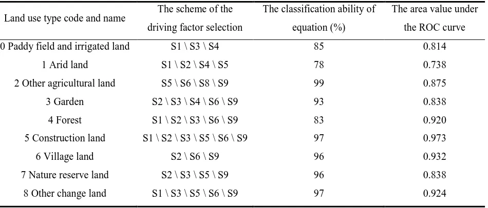
from land use type to driving factor, and the area value under the ROC curve is used to determine the relation-ship from driving factor to land use type, the regression equation which the area value under the ROC curve is the most should be selected, and the regression parame-ters of the equation should be recorded and entered into the file named alloc1.reg (regression results). Table 3 is the summary of the selection scheme to different land use type and its classification ability of equation and area value under the ROC curve.
Table 3.The summary of the driving factor selection
Land use type code and name The scheme of the driving factor selection
The classification ability of
equation (%)
The area value under
the ROC curve
0 Paddy field and irrigated land S1 \ S3 \ S4 85 0.814
1 Arid land S1 \ S2 \ S4 \ S5 78 0.738
2 Other agricultural land S5 \ S6 \ S8 \ S9 99 0.875
3 Garden S2 \ S3 \ S4 \ S6 \ S9 93 0.838
4 Forest S1 \ S2 \ S3 \ S6 \ S9 83 0.920
5 Construction land S1 \ S2 \ S3 \ S5 \ S6 \ S9 97 0.973
6 Village land S2 \ S6 \ S9 96 0.932
7 Nature reserve land S2 \ S3 \ S5 \ S9 96 0.838
8 Other change land S1 \ S3 \ S5 \ S6 \ S9 97 0.924
It can be obtained from table 3 that both the classifica-tion ability of equaclassifica-tion and the area under the ROC curve related to different land use types is higher than 70% and 0.7. Among all the 9 land use types, 4 land use types‟ ROC
value is higher than 0.9, and 4 land use types‟ ROC value
is higher than 0.8. Therefore, the model has a strong ex-planatory ability.
5) Change matrix and elastic coefficience
Coefficient matrix and elastic are set up in order to de-termine the rule and order of the mutual transformation among the different land use types.It also needs to analyze the present situation of the land use in the study area con-cretely. Before simulating the change of the land use, the change matrix should be entered into the file named al-low.txt, and the elastic coefficience should be entered into the main parameter file named main.1.
According to the characteristics and change policies of the study area, „the other unchanged land use type‟ is set in the change matrix, which cannot be transformed to any other land use type or transformed from any other land use type, „reservations land‟ is set, which cannot be trans-formed to any other land use type, and „paddy filed and irrigated land‟ is set which cannot be transformed to „ con-struction land‟. Other values in a matrix are set to 1, as
convertible relationship. 6) Main parameter file
The file named main.1 contains a set of 20 parameters, such as the number of land use types or the max number of independent.
4.3.
Simulating the land use
When the prepared data are stored in the CLUE-S model‟s installation path, open the user interface of the CLUE-S model, select a region restricted file and a demand file for
land use, then click “run” to start the simulation. If there are some errors in the simulation process, the error can be corrected with reference to the problem in the log file.
5.
Results analysis
Simulation of Land-Use Policies on Spatial Layout with the CLUE-S Model 5
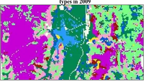
Depending on the Figure 1 (a) and (b), analyze the change condition of the spatial layout of the nine land use types between 2009 and 2015 comparatively, combined with the policy analysis of the study area, these results could be obtained.
1) The original spatial layout of the towns is changed, but the land use is still concentrated as before, the area of the towns increases a little, and the overall layout is moved to the east. A portion of the land which belonged to the towns before has transformed into paddy field and irrigated land. At the same time, a part of village land which was once used by the towns is spared, and a part of forest land which was one used by the towns is also spared from the flat terrain area to the gentle slope. As discussed before, the simulation results reflect the land use policies of the experimental area like „centralized layout‟, „the intensive use of land‟, „construction land up the hill‟, „towns provid-ing land for plough (low mound and gentle slope)‟ and
„construction land development along the river and road‟. 2) The village land area increases a little, and the layout is more concentrated. The village land scattered in paddy field and irrigated land originally is transferred to the
side‟s edge on the west and east of the paddy field and i r-rigated land. This change is accorded with the demands of the land use policies of this area like „centralized layout‟ and „the intensive use of land‟.
3) Garden area increases to a great extent, which is in accordance with land use policy „newly increase flower area 609 hectares‟. Most of the new garden occupies the original forest land, with its spatial layout of dry land and its future developing along the highway trend. This change meets the needs of flower products for export.
4) Cultivated land area is increases 232 hectares, which is in accordance with the requirement of the land use poli-cy.
5) Natural reservation area reduces a little, much of which is transformed to forest. This change meets the de-mand of the land use.
In summary, the experimental results are consistent with the experimental purpose. The simulation experiment could simulate the main change of the land use on the basis of the land use policies of the study area.
Figure 1(a) spatial layout distribution grid of nine land use
types in 2009
Figure 1(b) spatial layout distribution grid of nine land use types in 2015.
6.
Conclusion
The land use change simulation is greatly influenced by land classification and the selection of driving factors corresponding to the different land use types. Therefore, in the simulation of the land use change based on the land use policies of the study area, this paper use Arc GIS software to analyze the structure and the spatial layout of the current land use situation of the study area at first, in order to ana-lyze the dynamic demand of the land use according to the major land use change policies of the study area in the simulated year. Then, on the basis of analyzing the current land use situation and main land use change policies, the land use type is classified reasonably. After that, repeatedly screen the driving factors by using logistic regression model and ROC curve value, in order to choose the most suitable driving factors for the eventual land use character-istics of the study area. Finally, make the reasonable simu-lation through CLUE-S model for the spatial layout change based on the changes in the land use policies.
The results show that choice of the suitable parameters and driving factors according to the characteristics of the study area could make the simulation process more smoothly and the simulation accuracy higher. This paper realizes using the CLUE-S model to simulate the spatial layout change of the land use based on the land use poli-cies like „construction land up the hill‟, „towns providing land for plough‟, „construction land developing along the river and road‟, „important industrial land expansion‟,
„centralized layout‟ and „the intensive use of land‟ at the same time. The research results have certain significance to explore the change of the spatial layout like analyzing the land use change or the planning land use.
7.
Acknowledgments
REFERENCES
[1] Zhang Yongmin, Zhou Chenghu, Zheng Chunhui. Spatial Land Use Patterns in Guyuan County: Simu-lation and Analysis at Multi-Scale Levels. Resources Science, 2006, 28(2): 88-96
[2] Bai Wanqi, Zhang Yongmin, Yan Jianzhong. Simulation of land use dynamics in the upper reaches of the Dadu river. Geographical Research, 2005, 24(2): 206-214
[3] Pei Bin, Pan Tao. Land Use System Dynamic Modeling: Literature Review and Future Research Direction in China. Progress in Geography, 2010, 29(9): 1060-1066
[4] Tang Zhihua, Zhu Xianlong, Li Cheng. Analysis of Land Use/Land Cover Change in Yangzhou City Based on CLUE-S Model. Journal of Geo-Information Science, 2011, 13(5): 695-700
[5] Yu Shuyuan, Xi Yantao, Niu Kun, Yu Xuetao. CLUE-S Model of Land Use Change Simulation of Xuzhou City. Geospatial Information, 2010, 8(6): 103-107
[6] Guo Yanfeng, Yu Xiubo, Jiang Luguang, Zha Liangsong.
Scenarios analysis of land use change based on CLUE model in Jiangxi Province by 2030. Geographical Research, 2012, 31(6): 1016-1028
[7] Wu Jiansheng, Feng Zhe, Gao Yang, Huang Xiulan, Liu Hongmeng. Recent Progresses on the Application and Im-provement of the CLUE-S Model. Progress in Geography, 2012, 31(1): 3-10
[8] Liang Youjia, Xu Zhongmin, Zhong Fanglei. Land use scenario analyses by based on system dynamic model and CLUE-S model at regional scale: A case study of Ganzhou district of Zhangye city. Geographical Research, 2011, 30(3): 564-576
[9] Verburg PH, Soepboer W, Veldkamp A, Limpiada R, Es-paldon V, Mastura SS. Modeling the spatial dynamics of regional land use: the CLUE-S model. Environmental Management. 2002, 30(3): 391-405