Economics of Education Review 19 (2000) 1–15
www.elsevier.com/locate/econedurev
The effects of ability grouping on student achievement and
resource allocation in secondary schools
Julian R. Betts
a,*, Jamie L. Shkolnik
baDepartment of Economics, University of California, San Diego, La Jolla, CA 92093-0508, USA bNational Opinion Research Center, 1350 Connecticut Avenue, Suite 500, Washington, DC 20036, USA
Received 1 February 1996; accepted 1 January 1998
Abstract
A school policy of grouping students by ability has little effect on average math achievement growth. Unlike earlier research, this paper also finds little or no differential effects of grouping for high-achieving, average, or low-achieving students. One explanation is that the allocation of students and resources into classes is remarkably similar between schools that claim to group and those that claim not to group. The examination of three school inputs: class size, teacher education, and teacher experience, indicates that both types of schools tailor resources to the class ability level in similar ways, for instance by putting low-achieving students into smaller classes. [JEL I21]1999 Elsevier Science Ltd. All rights reserved.
Keywords:Educational economics; Educational finance; Human capital; Resource allocation
1. Introduction
The value of ability grouping in schools is a subject of much debate. Supporters of ability grouping argue that there are efficiency effects to be gained for all students by putting similar students into classes that can be tail-ored to their abilities. However, opponents of ability grouping argue that there are also peer group effects so that the achievement of a given student depends not only on his or her initial ability, but also on the average ability of the class. Thus, having high-achieving and motivated students in the class raises everyone’s level of achieve-ment, and by grouping, schools essentially harm the lower ability students by separating them from the high ability students. The peer group effect includes potential harm done to test scores of low ability students due to lowered expectations and self-esteem.
Previous research using large data sets can be classi-fied into three types (for a review of the ethnographic
* Corresponding author. Tel.:11-415-291-4474; fax: 1 1-415-291-4401; e-mail: [email protected]
0272-7757/99/$ - see front matter1999 Elsevier Science Ltd. All rights reserved. PII: S 0 2 7 2 - 7 7 5 7 ( 9 8 ) 0 0 0 4 4 - 2
research, see Gamoran & Berends, 1987). The first type of study compares students in the academic track to those in the same school who are in the general and/or the vocational track. The second type compares students in schools that group to students in non-grouped schools. A third and more recent approach compares students in high, middle, and low ability groups to ungrouped or heterogeneously grouped students (ungrouped and het-erogeneously grouped are used interchangeably).
Studies that compare high to low groups overwhelm-ingly find that those in high groups have higher math achievement (see Alexander & McDill, 1976; Gamoran, 1987; Vanfossen, Jones & Spade, 1987, for example). Gamoran (1987) uses the vocational track as the omitted category and finds much within-school variation. Even studies that conclude that ability grouping has no effect on a variety of student outcomes find effects of ability grouping on math achievement growth (see Jencks & Brown, 1975; Alexander and Cook, 1982).1 Although
many studies of this type control for initial ability by including lagged test scores, types of courses taken, soci-oeconomic status, and other background variables, it is likely that there are other factors such as motivation and effort that affect both group placement and math achievement.
One solution, used in the second type of study outlined above, is to compare mean achievement of students in schools that use homogeneous grouping to that of stu-dents in schools with heterogeneous grouping. Slavin (1990) finds that ability grouping has little or no overall effect on achievement. However, Hallinan (1990) notes that the studies reviewed by Slavin compare the mean
achievement growth in each type of school, not the dis-tribution. She argues that if there are differential effects to grouping, then when high ability students gain and low ability students lose, the net effect could still be zero.
Ideally, we want to assess how the students in the vari-ous levels of grouped classes would fare if they were moved to heterogeneous classes. The third type of study in the literature attempts to address this problem by com-paring students in each of the different ability group lev-els to students in heterogeneous classes. Using British data, Kerckhoff (1986) compares high, middle, low, and remedial students at grouped schools to a reference cate-gory of ungrouped students, using several lagged test scores to control for initial ability. He finds evidence for the differential effects theory: students in the high ability class do better than the average student at an ungrouped school, and students in a low ability class at a grouped school do worse than the average student at an ungrouped school. Hoffer (1992) and Argys, Rees and Brewer (1996) also find evidence for differential effects. Hoffer (1992) uses Longitudinal Study of American Youth (LSAY) data to compare high, middle, and low grouped classes to heterogeneous classes. He finds that being in a high group has a positive effect and being in a low group has a negative effect, with a net effect of zero. In order to compare the high grouped students to their counterparts at a non-grouping school, he uses a propensity score method, in which he runs an ordered probit to model group selection using only the grouped schools, and then using the resulting coefficient esti-mates, calculates a propensity score for heterogeneously grouped students as well as the homogeneously grouped students. He ranks the students based on their propensity scores and then divides them into quintiles. In this way,
English achievement, and American history achievement, while finding effects on quantitative SAT, senior year educational plans, and application to college. Jencks and Brown (1975) find little effect on vocabulary, total information, reading compre-hension, abstract reasoning, and arithmetic computation, while finding effects on arithmetic reasoning.
he can compare grouped and non-grouped students who have similar backgrounds and who thus fall into the same propensity quintile. He runs a separate regression for each quintile, but within the quintile he again compares high, middle, and low grouped students to the average heterogeneously grouped student, and again finds evi-dence for differential effects of grouping.
Hoffer’s indicator for grouping is based on teacher interviews, school documents, and when necessary, phone calls to the schools. He divides students into four groups: high, medium, and low ability classes in grouped schools, andallstudents in schools which claim not to use ability grouping. Although teachers at all schools in his sample report on class ability, Hoffer categorizes classes in non-grouped schools as heterogeneous. The students at non-grouping schools are the control group against which he compares the progress of students in classes at the three ability levels at grouped schools. Here, we argue, it might be better to compare grouped to non-grouped students within class ability levels, since teachers’ observations of class ability may do more to control for unobserved heterogeneity than even the pro-pensity score method.
Argys, Rees and Brewer (1996) also use a two step procedure to account for selectivity into the various classes. Their first step is a multinomial logit for group placement, using high, middle, and low grouped classes, with the heterogeneously grouped students as the omitted category. From the multinomial logit model, they obtain an inverse Mills ratio for each observation, and include it in the separate test score regressions for each of the four groups. They calculate predicted achievement for each group, and also find differential effects: grouping helps the above average and average students, but harms the below average students, as compared to the hetero-geneously grouped students. Argys, Rees, and Brewer address not only the differential effects of ability group-ing, but also the other important question in the litera-ture: the overall mean effect of ability grouping on achievement. They conclude that ability grouping has a small positive net effect on achievement.
In sum, past studies which compare students from dif-ferent ability groups to heterogeneously grouped students find evidence that the top students are helped by ability grouping and the bottom students are harmed, resulting in a net effect that can be positive or negative, but which is usually close to zero.
The goal of this paper is to analyze both the overall effect and the differential effects of a formal policy of ability grouping. Ideally, one would like to compare high ability students at grouping schools to their high ability counterparts at non-grouping schools, and likewise for middle and low ability students. Accordingly, this paper furthers the research by controlling for class ability at
this paper is the examination of one of the most important criticisms of ability grouping, that ability grouping leads to inequality in inputs (class size, teacher education, and teacher experience) among classes, as suggested by Oakes (1990). We model the allocation of resources among classes in a given school and test whether schools that group use resource allocation to exacerbate existing inequalities. The study of how ability grouping alters intra-school allocation of resources is useful for a second reason: since one of the main theor-etical advantages of ability grouping is that it allows schools to tailor the mix of school inputs such as class size and teacher qualifications to the needs of different types of students, it is important to know the extent to which schools vary inputs by class.
2. Empirical model
We address two questions concerning the effect of for-mal ability grouping on student achievement. First, does ability grouping increase student achievement on aver-age? Second, does ability grouping have varying effects on achievement depending on the initial level of class ability or student ability?
The first model tests the net effect of ability grouping. Do students in grouped schools fare better, on average, than students in non-grouped schools? The model is the prototypical education production function (this is typi-cally a linear function):
Sit5f(Sit21,Fi,Xit,Tit),2 (1)
where Sit5achievement, math test score for individual
i at time t; Sit−1 5 initial achievement or ability, i.e.
initial math test score; Fi 5 background, {race, sex,
urban, region, parents’ education levels}; Xit 5 school
inputs, {teacher–pupil ratio, teacher experience, teacher education}; andTit5grouping dummy51 if student’s
school groups in math classes. If grouping is beneficial, the coefficient will be positive and significant.
Hoffer (1992) supplements this model with a second model which compares three ability levels in grouping schools, high, middle, and low, to a control group of all students in ungrouped schools to determine who receives the benefits. In this model,
Sit5f(Sit21,Fi,Xit,Hit,Mit,Lit), (2)
where Hit, Mit, and Lit are dummy variables for high,
2Total achievement is a function of not only the inputs at timet, but of all prior inputs:
Sit5f(Fit,Fit21,...,Fi1;Xit,Xit21,...,Xi1;Tit,Tit21,...,Ti1). Since these prior inputs are unobserved, we substitute Sit215f(Fit21,...,Fi1;Xit21,...,Xi1;Tit21,...,Ti1) into the
equ-ation forSitto control for past inputs.
middle, and low ability classes in grouped schools. If the coefficients are all positive or zero, then proponents of ability grouping are right and there is no support for the claim that ability grouping harms some students. Hoffer finds negative coefficients on the low and middle groups and positive coefficients on the high groups, all signifi-cant at the 5% level, and concludes that this indicates differential effects of ability grouping, with gains for stu-dents in high ability classes at the expense of those in the lower ability classes. However, in this specification, the control group consists of all students at ungrouped schools. Thus it compareshigh abilitystudents at group-ing schools to theaveragestudent at ungrouped schools and finds higher achievement gains for the former. We argue that group placement may be correlated with unob-served motivation and effort, and so the coefficients on class ability level in the grouping schools may be biased. To see this point, assume that in reality grouping has no effect onany student’s achievement, so that a stud-ent’s peer group, or class ability level, has no causal effect on his or her rate of learning. But suppose at the same time that part of the error term is unmeasured motivation of the student. Let the student’s unobserved ability or motivation be captured by a continuous vari-ableMOTit. It seems reasonable that the teacher’s
identi-fication of the student’s class ability, which is summar-ized in theHit,Mit, and Litvariables, is correlated with
the student’s own motivation, which is unobservable to the econometrician. For instance, the following corre-lations might obtain:r(MOTit,Hit) > 0,r(MOTit,Mit)5
0, andr(MOTit,Lit),0. Then suppose we run the
fol-lowing regression,
Sit5c1Sit21a 1Fib 1XitG 1HituH (2a)
1MituM1LituL1(MOTit1eit)
where each of theucoefficients is in truth zero, and the final two terms in parentheses represent the compound error term. The OLS estimates of the impact of class ability in grouped schools are likely to be biased, indicat-ing that groupindicat-ing aggravates inequality in student achievement. That is, the estimate ofuHis likely to be
positive and the estimate ofuLis likely to be negative,
even though in the true data generation process both coefficients are zero. The bias occurs because the class ability variables are likely to be correlated with unob-served student motivation or ability. We would argue that a useful check is to extend Eq. (2) to include meas-ures of class ability in both grouped and ungrouped schools. We will expand on this point below.
Argys, Rees and Brewer (1996) estimate separate OLS achievement equations for each of the following four groups: above average, average, below average, and het-erogeneously grouped students, wheres denotes a stud-ent’s group placement,
If group placement and achievement are both corre-lated with the unobserved characteristics, then the achievement equation without corrections will yield biased results. They include a selectivity correction to account for the fact that students are placed into groups based on unobservable student traits like motivation, which are likely to also be correlated with achievement. Here,ldenotes the inverse Mills ratio, a selectivity cor-rection calculated from a multinomial logit model of ability group placement. This model will be unbiased if the selectivity correction succeeds in controlling for omitted variables which are correlated with ability group placement.
Our paper adds another model to the literature by con-trolling for class ability level in the non-grouping schools as well. The model becomes:
Sit=f(Sit−1,Fi,Xit,THit,TMit,TLit,NHit,NMit,NLit),
(3)
where the prefix T indicates grouping and N indicates non-grouping schools. The grouping variable is derived from a question which asks the school principal whether the school uses grouping in math classes. High, middle, and low groups are denoted by the suffixes H, M, and
L. Here, we run three separate regressions, each omitting eitherNHit,NMit, orNLitas the control group. The null
hypothesis in each regression is that the coefficient on the corresponding dummy variable, THit,TMit, or TLit,
is zero. If we cannot reject the null, then grouping has no effect on the group in question. If a coefficient is positive (negative), then grouping is beneficial (detrimental) to the group.
This specification is likely to reduce the potential for omitted variable bias. Since the correlation between unobserved motivation and ability and the teacher’s esti-mate of class ability is likely to be similar in schools with and without grouping, we can use the difference in the class ability coefficients between the two types of schools to identify the effect of being placed in a given ability group in a school that groups. In other words, we improve on model Eq. (2a) by sweeping out of the error term the part ofMOTitwhich is correlated between
stu-dents who are in classes of the same ability, but who in one case are in grouped schools and in other cases are in ungrouped schools. By using the proper control group in Eq. (3), we can determine whether the results in model 2 are influenced by the comparison of the different types of students in addition to the two types of schools. We test for an overall effect of ability grouping by estimating Eq. (1) and differential effects of ability grouping using Eq. (3), which provides a more meaningful comparison than Eq. (2).
3. Data
The data set is from the Longitudinal Study of Amer-ican Youth (LSAY), a national study which follows two cohorts of students from approximately 100 middle schools and high schools from 1987 to 1992. Students first begin the study in grades 7 or 10, so our data cover grades 7 through 9 for one cohort, and grades 10 through 12 for the other. Surveys completed by principals, teach-ers, students, and parents provide detailed information on student and teacher background characteristics at the classroom level. This paper uses 5442 observations on students, their teachers, their classrooms, their test scores, and their schools to estimate the effects of ability grouping. We use the first three years of data since teach-ers’ estimates of class ability are available for only these years (for a review of the LSAY data-set, see Miller, Hoffer, Suchner, Brown & Nelson, 1992).
The variables can be divided into five main categories:
1. Achievement: Students take standardized math tests at the beginning of each school year. Initial achieve-ment,St−1, is distinguished from achievement, which
is measured by St, representing attainment up to and
including time t. By controlling for initial achieve-ment, we can estimate the effect of the school inputs on achievement over yeart.
2. Family Background: The model controls for back-ground variables which are likely to affect test scores, i.e. race dummies for black, Asian, Hispanic, and Native American, a dummy for sex, dummies indicat-ing whether the school is suburban or rural, dummies for three of four regions, and four of five dummies for parents’ education levels.
3. School Inputs: The school inputs considered are the main components of school expenditures: teacher– pupil ratio,3 number of years of teacher experience,
and education level of the teacher,4all for the
stud-ent’s actual math class. An increase in any of these is likely to lead to an increase in school expenditure. 4. Ability grouping: The principal reports whether the school uses “ability grouping or tracking (other than AP courses)” (where AP stands for Advanced Place-ment classes) in its math classes. Grouping is a dummy variable equal to one if the student’s school groups in math classes and zero otherwise. Twenty-seven percent of the observations in this sample are from schools that claim not to use ability grouping in math classes. This variable is different from Hoffer’s, which uses information from teachers, school
docu-3Teacher–pupil ratio is used in lieu of class size because teacher–pupil ratio is positively related to school expenditure.
ments, and phone calls. In his sample, 15% of the students in seventh grade math classes are in schools that do not group students by ability. This variable was not available to us.
5. Class Ability Level: Class ability is measured in two ways. The first way is similar to Hoffer’s and defines class ability as measured by the teacher’s evaluation of the average ability level of the class compared to other classes in that school, from 1 (lowest) to 5 (highest).5,6This variable is especially useful because
it is available not only for grouping but for non-grouping schools. It allows us to compare student test scores as well as available school inputs in classes of similar ability across school types, which leads to interesting and instructive results. If the non-grouped classes are mainly heterogeneous, we would expect to see most of them in the average class ability group.
The second measure of class ability level is calculated by demeaning initial achievement for each student by grade level and then grouping students based on the quartile of their demeaned scores. We assume that in a grouping school a student’s ability level will be highly correlated with class ability level, while in a non-group-ing school, a student’s own ability level will not be parti-cularly correlated with class ability level if classes are heterogeneous. The ability quartile measure is possibly a less accurate gauge than the teacher’s evaluation, but is also less subjective and supports the results. All three models will be estimated for both class ability measures.
4. Results
4.1. Achievement growth
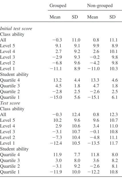
To show that class ability groupings are comparable between the two school types, Table 1 presents means and standard deviations for initial test scores and for test scores by school type and by both measures of class ability level. Initial test scores increase steadily as the class ability level increases. Surprisingly, the mean test scores seem comparable between the two types of schools, both overall and within ability groups. More-over, the standard deviations of test scores within ability groups are remarkably similar between schools with and without grouping.
To portray the composition of students across ability
5The question reads, e.g. for seventh grade teachers, “How would you rate the average academic ability of the students in this class compared to all 7th graders in your school?” Answers include: much higher than average, somewhat higher, about average, somewhat lower, and much lower than average.
6This class ability variable is available for the first three years of the survey.
Table 1
Means and standard deviations (SD) of test scores for grouped and non-groupedaby class ability levelband by ability quartilec
Grouped Non-grouped
Quartile 4 13.2 4.4 13.3 4.6
Quartile 3 4.5 1.8 4.7 1.8
Quartile 4 11.9 7.7 11.8 8.0
Quartile 3 3.0 8.0 3.6 8.2
Quartile 2 23.1 9.2 22.6 8.1
Quartile 1 211.9 10.0 212.2 10.8 aTest scores are demeaned by grade level.
bClass ability level is determined by the teacher (55highest). cAbility quartiles are based on initial test scores demeaned by grade level.
non-Table 2
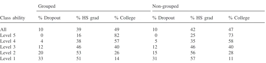
Composition of students in grouped and non-grouped schools by class ability level
Grouped Non-grouped
Class ability % Dropout % HS grad % College % Dropout % HS grad % College
All 10 39 49 10 42 47
Level 5 0 16 82 0 25 73
Level 4 4 38 57 5 35 58
Level 3 12 46 40 12 46 40
Level 2 20 53 26 15 56 28
Level 1 33 51 14 31 57 11
grouping schools among the lower levels of classes. In schools that used grouping, teachers report that they expect slightly more students to drop out in the lowest ability classes.
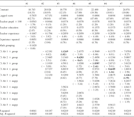
Table 3 shows the test score equations where we group students by class ability level. In the first regression, which includes all of the control variables and the group-ing dummy, the groupgroup-ing coefficient is not significantly different from zero, with at-statistic of 20.48. So, on average, students at grouping schools do neither better nor worse than students at non-grouping schools.
Regression 2 is similar to the Hoffer specification where, instead of the grouping dummy, we include inter-action terms between each class ability level and group-ing; there are five dummies for class ability level in the grouping schools and the comparison group consists of the heterogeneously grouped students who attend non-grouping schools. These terms are almost all significant in the expected direction. Class ability levels 1, 2, and 3 are all negative and statistically significant at the 1% level, which seems to indicate that students in classes of average or below average class ability will learn less when a school groups by ability. The students in above average levels 4 and 5 in grouping schools seem to learn at significantly higher rates. Moreover, the coefficients increase monotonically with class ability in the grouped schools.
Since we have information on the class ability levels in the non-grouping schools as well, it is useful to com-pare level 1 grouped classes to the level 1 classes at non-grouping schools. As we argued earlier, using students in classes at a similar ability level in non-grouped schools as the control group, rather than all students at non-grouped schools, is likely to reduce omitted variable bias due to unobserved ability or motivation. To the extent that this is a problem in the data, we would expect regression 2 in the table to overstate the gap in learning across ability groups. Regressions 3 through 7 each include 9 of the 10 dummy variables for the interaction between the five class ability levels and the grouping dummy variable. Each regression excludes one of the (class level3non-grouping variables). So, for instance,
in regression 3, to test if a level 1 grouped class is stat-istically different from a level 1 non-grouped class, we examine the coefficient on (level 1 3 grouping). The relevant coefficients and t-statistics are in bold. In regressions 3 and 4, we see that the coefficients for levels 1 and 2 are statistically insignificant at the 5% level. This indicates that it is no worse to be in a lower ability level class in a grouping school than in a non-grouping school, contradicting the results in model 2 where the compari-son group consisted of all ‘heterogeneously grouped’ classes. The average classes, however, fare worse in grouping schools, as shown in regression 5. The coef-ficient is negative and statistically significant at the 2% level. Finally, regressions 6 and 7 estimate the effect on the two top ability groups, where neither coefficient is significant at the 5% level, indicating that students in these classes do not benefit substantially from grouping. The coefficient on the top grouped students is positive, and marginally significant with ap-value of 0.07.
Models 3–7 indicate very different results to those in model 2, where the comparison group was all students in non-grouping schools. In model 2, the difference in achievement gains over one year ranges from a loss of 4.2 points for the lowest group, to a gain of 3.2 points, a difference of 7.4. This range is quite large compared to the average test score gain in the full sample of 2.3 points per year. In the new specifications, the difference in test score gains ranges from a loss of 1 point in the middle ability group to a marginally significant gain of 1.1 in the top group, for a total of 2.1 points. This gap is significantly less than the 7.4 point difference in model 2 and previous models.7
Table 3
OLS results for regressions of test scores on class ability levelsa
#1 #2 #3 #4 #5 #6 #7
Constant 16.743 20.926 16.770 20.333 22.400 24.033 24.974
(16.33) (18.95) (12.15) (17.89) (19.56) (19.81) (19.08)
Lagged score 0.7835 0.7151 0.6894 0.6894 0.6894 0.6894 0.6894
(62.71) (50.60) (47.69) (47.69) (47.69) (47.69) (47.69)
Teacher–pupil3100 20.0543 20.0044 0.0378 0.0378 0.0378 0.0378 0.0378
(21.79) (20.15) (1.20) (1.20) (1.20) (1.20) (1.20)
Teacher education 0.5742 0.3483 0.1575 0.1575 0.1575 0.1575 0.1575
(2.07) (1.28) (0.59) (0.59) (0.59) (0.59) (0.59)
Teacher experience 20.1687 20.1794 20.2059 20.2059 20.2059 20.2059 20.2059 (23.63) (23.92) (24.49) (24.49) (24.49) (24.49) (24.49)
Experience squared 0.0051 0.0057 0.0068 0.0068 0.0068 0.0068 0.0068
(3.55) (3.96) (4.76) (4.76) (4.76) (4.76) (4.76)
Math grouping 20.1420 (20.48)
Cl Ab 13group 24.2181 1.1249 22.4375 24.5049 26.1375 27.0788
(26.62) (1.02) (23.10) (26.66) (28.01) (28.27)
Cl Ab 23group 22.3665 3.1340 20.4283 22.4958 24.1284 25.0697
(25.51) (3.08) (20.67) (25.06) (26.99) (27.32)
Cl Ab 33group 21.1019 4.5911 1.0288 21.0387 22.6713 23.6126
(23.08) (4.54) (1.72) (22.41) (25.01) (25.61)
Cl Ab 43group 0.7237 6.6019 3.0395 0.9721 20.6605 21.6018
(2.04) (6.45) (4.98) (2.25) (21.26) (22.56)
Cl Ab 53group 3.2130 9.3299 5.7675 3.7001 2.0675 1.1262
(8.04) (8.82) (8.77) (7.79) (3.77) (1.79)
Cl Ab 13nogrp 23.5624 25.6298 27.2624 28.2037
(23.24) (25.45) (26.72) (27.19)
Cl Ab 23nogrp 3.5624 22.0674 23.7000 24.6413
(3.24) (23.25) (25.28) (25.84)
Cl Ab 33nogrp 5.6298 2.0674 21.6326 22.5739
(5.45) (3.25) (22.94) (23.91)
Cl Ab 43nogrp 7.2624 3.7000 1.6326 20.9413
(6.72) (5.28) (2.94) (21.35)
Cl Ab 53nogrp 8.2037 4.6413 2.5739 0.9413
(7.19) (5.84) (3.91) (1.35)
R-squared 0.6041 0.6187 0.6249 0.6249 0.6249 0.6249 0.6249
Adj.R-squared 0.6020 0.6165 0.6224 0.6224 0.6224 0.6224 0.6224
aClass ability level is determined by the teacher (55highest).
Includes school inputs. Hetero-robustt-statistics in parentheses.N55442.
Other regressors included but not shown: dummies for grade level, race, sex, region, parents’ education levels, and whether the school is suburban or rural. See the data section for a more detailed description.
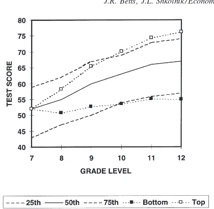
The standard specification in model 2 predicts a gap of 7.4 points per year in attainment between identical students who are placed into the top and bottom classes. To gauge whether this prediction is realistic, we plot in Fig. 1 actual test scores by grade level in our sample. The solid line indicates the median score, and the two dashed lines indicate the 75th and 25th percentile scores. We superimpose on this what would happen to two identical students who performed at the median level at the start of grade 7 if one were placed in the bottom level class of a grouping school and the other were placed in the top level class of a grouping school. The dotted lines
with white and black boxes indicate the predicted tra-jectory for the student in the top class and the student in the bottom class respectively. Thus, after one year, their test scores are predicted to have diverged by 7.4 points.8Note that after only three years, one of the two
8In later years, we calculate divergence from the median student score by adding to the median student score (11r 1
Fig. 1. Actual range of test scores, and predicted scores of identical individuals placed in top and bottom classes.
students, who was initially at the median test score, has fallen below the 25th percentile, while the student placed in the top ability class has risen above the 75th percen-tile. We find these predicted effects too large to be cred-ible. After all, if grouping had such large differential effects, we would expect to see widening inequality in student achievement as students get older. However, as shown by the nearly parallel lines depicting the 25th and 75 percentile scores in the empirical distribution, the dis-persion of test scores widens very slowly in the higher grades, supporting our contention that earlier work may overstate the differential effects of ability grouping, per-haps due to omitted variable bias.9
If ability grouping affects a particular school’s allo-cation of inputs among classes, then the input levels are endogenous. The exclusion of the potentially endogen-ous classroom inputs from the models in Table 3 yields reduced form equations. If grouping improves perform-ance by allowing schools to tailor specific inputs to each class, the grouping coefficient will be greater in the reduced form, since now the grouping variable will
cap-9The predicted gap of 7.4 points in test scores between a student placed in the bottom and top tracks after only one year is very close to what is found by Hoffer (1992) and Argys, Rees and Brewer (1996). Hoffer (1992, Table 3) reports that in Grade 7 classes the predicted differential is 6.0 points for Grade 7 math (out of a score of 100 as in our work), while Argys, Rees and Brewer (1996, Table 4A) report that the average student, if placed in the bottom or top track of a school with tracking, would obtain test scores 5.0 points below or 5.8 points above the score he or she would obtain if in a non-tracked class. (This math test score is also out of 100). This yields an even larger predicted gap of 10.8 points between identical students placed in the top and bottom tracks.
ture these effects, if they exist. If grouping causes differ-ential effects by allocating more and better resources to top ability groups at the expense of the lower ability groups, it will be reflected in lower coefficients for the bottom groups and higher coefficients for the top groups. The coefficients and t-statistics in the reduced form change little, however, indicating that the difference in resource allocation between the two types of schools is either small or ineffectual. The results are similar when these models are repeated using achievement quartiles instead of mean class ability.10,11
What are we to conclude from these results? First, the first regression in Table 3 indicates that the net overall effect of formal ability grouping in math on theaverage
student is insignificantly different from zero. We thus largely agree with Hoffer (1992), who found no signifi-cant effect and Argys, Rees and Brewer (1996), who did find a positive and significant but small effect.
The second and more controversial question in the literature concerns whether ability grouping causes the students with higher initial achievement to learn at a fas-ter rate, and those with lower achievement to learn less quickly than students without grouping. We can replicate the results of Hoffer (1992) and Argys, Rees and Brewer (1996) quite closely, in the sense that using a similar specification we find evidence of very large differential effects. However, when we use students in similar ability groups in non-grouped schools as the control group, we find much smaller differential effects. We believe that this alternative specification greatly reduces omitted ability bias that is likely to exaggerate the differential effects of grouping. Nevertheless, we still find some evi-dence of differential effects of grouping, even in the alternative specification. The results seem to confirm the finding by Hoffer (1992) and Argys, Rees and Brewer (1996) that grouping can aggravate inequality in achieve-ment, but we find that the gap in rates of learning between the top and bottom classes is much smaller than reported by these earlier papers. In sum, our results are in fact closer to those of Hoffer (1992) and Argys, Rees and Brewer (1996) than to those of Slavin (1990) who concludes that there are no differential effects of group-ing.
4.2. Robustness tests
We perform robustness tests that confirm the results found in Table 3. First we run separate regressions for
10Quartile group placement is based on the ranking among all students of an individual student’s initial test score determ-ined by grade level.
each of the class ability levels.12Next we calculate
pro-pensity quartiles and run four separate regressions. Finally, we control for the selection of students into ability groups using 2SLS.
4.2.1. Regressions by class ability level
The estimation of separate regressions for each of the five ability groups achieves a less restrictive model, although it reduces sample sizes. These regressions include only a portion of the sample, so we include selec-tivity corrections in the form of an inverse Mills ratio in the test score equation. We generate the inverse Mills ratio using an ordered probit model that allows us to account for the ordinal nature of the class ability variable in a way that the multinomial logit cannot (see Greene, 1993). The underlying model is
C*5bX1e,
whereXis the set of explanatory variables, andeis the residual.C* is an unobserved latent variable, but we can determine to which category it belongs. We observe:
C51 ifC*#0,
C52 if 0,C*#m1,
C53 ifm1,C*#m2,
C54 ifm2,C*#m3,
C55 ifm3#C*.
Thems are unknown parameters estimated jointly with
b. A list of variables and results are shown in Table 4. We use three additional instruments to identify the stud-ent’s placement into ability group: the percentage of dents who are black in the school, the percentage of stu-dents who receive full federal lunch assistance at the school, and the student’s test score relative to the average for his or her grade. The justification for these instru-ments is that the student’s own relative achievement and the demographic traits of the student body are likely to be correlated with his or her relative standing within the school, and hence the achievement of the class to which the student is assigned. Each is a highly significant pre-dictor of ability group. The second set of results shown in the table shows results when the three instruments are excluded. A likelihood ratio test indicates that the three additional instruments are jointly significant at the 1% level. They are not significant in the test score equation, however, and make good instruments.
Each of the five test score regressions includes a dummy variable equal to one if the school groups and zero otherwise. The inverse Mills ratio, calculated from
12We would like to thank an anonymous referee for this suggestion.
Table 4
Ordered probit results for class ability levela
Regressors #1 #2
Constant 21.4014 21.4489
(29.63) (211.59)
Lagged test score 0.0083 0.0531
(0.45) (34.37)
Black 20.0816 0.0466
(21.41) (0.89)
Hispanic 20.1342 20.0978
(22.40) (21.76)
Asian 0.4654 0.4744
(4.38) (4.47)
Male 20.0613 20.0633
(22.08) (22.16) Teacher–pupil ratio 20.0681 20.0696
(29.80) (210.05)
Teacher experience 0.0207 0.0229
(3.23) (3.60)
Experience squared 20.0009 20.0010 (24.59) (25.01)
Log likelihood 27031.7 27049.9 aClass ability level is determined by the teacher (55highest). Hetero-robustt-statistics in parentheses. Column #1 was used for the propensity score and 2SLS analyses.N55442. Other regressors included but not shown: dummies for grade level, region, parents’ education levels, and whether the school is suburban or rural. See the data section for a more detailed description.
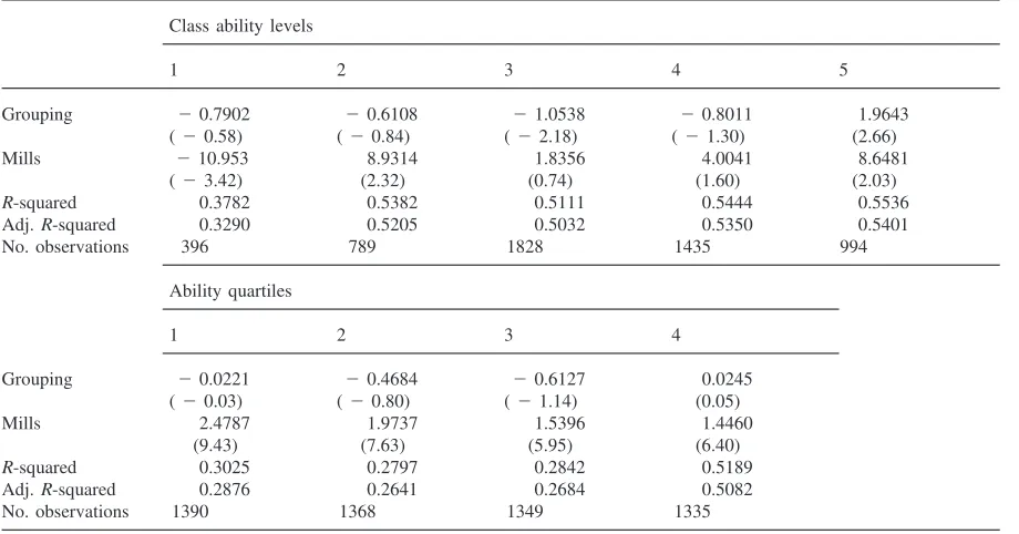
the ordered probit, is included to account for the selec-tivity in each of the subsample regressions. As shown in Table 5, for the two lowest groups the coefficients on the grouping variable are statistically insignificant. The next two higher groups are harmed by grouping, with a significant effect for the average group only. The top group is helped. The size of these predicted effects is fairly small. Regressions using achievement quartiles instead of mean class ability indicate that grouping has no effect on achievement at any level. We interpret this as limited evidence that a formal policy of grouping dif-ferentially affects math progress.
4.2.2. Regressions by propensity quartile
Table 5
OLS results for separate regressions of test scores on grouping by class ability levelaand ability quartileb Class ability levels
1 2 3 4 5
Grouping 20.7902 20.6108 21.0538 20.8011 1.9643
(20.58) (20.84) (22.18) (21.30) (2.66)
Mills 210.953 8.9314 1.8356 4.0041 8.6481
(23.42) (2.32) (0.74) (1.60) (2.03)
R-squared 0.3782 0.5382 0.5111 0.5444 0.5536
Adj.R-squared 0.3290 0.5205 0.5032 0.5350 0.5401
No. observations 396 789 1828 1435 994
Ability quartiles
1 2 3 4
Grouping 20.0221 20.4684 20.6127 0.0245
(20.03) (20.80) (21.14) (0.05)
Mills 2.4787 1.9737 1.5396 1.4460
(9.43) (7.63) (5.95) (6.40)
R-squared 0.3025 0.2797 0.2842 0.5189
Adj.R-squared 0.2876 0.2641 0.2684 0.5082
No. observations 1390 1368 1349 1335
aClass ability level is determined by the teacher (55highest).
bAbility quartiles are based on initial test score demeaned by grade level. Hetero-robustt-statistics in parentheses.
Other regressors included but not shown: lagged test scores, school inputs, school size, percent Hispanic, dummies for grade level, race, sex, region, parents’ education levels, and whether the school is suburban or rural. See the data section for a more detailed description.
class ability levels at the grouping schools, and assume that classrooms at non-grouping schools were hetero-geneous. Following the propensity score method of Rosenbaum and Rubin (1983), which was employed by Hoffer (1992) as described in the introduction, we include only the 3972 grouped-student observations in the first step (ordered probit model) and then calculate propensity scores for group placement for the full sample of 5442 observations.
We then divide the sample into quartiles based on the propensity scores, creating four groups of students of similar backgrounds, where the fourth quartile students are the most likely to be placed in a high level class. We test for the effects of grouping within each quartile by testing the significance of the coefficient of the grouping dummy. In Table 6, Models 1–4 show that the coef-ficients are insignificantly different from zero, indicating that grouping has no effect on the average student within a propensity quartile.
4.2.3. Two-stage least squares
Since the regressions in Table 3 use the entire sample, unlike the regressions in Table 5, they are not subject to selectivity bias. But the problem is transformed to one in which the dummies for class ability may be endogenous
functions of unobserved traits of the student. To deal with this possibility, we replicate model 2 in Table 3 substituting the probability of being in a particular class ability level for the actual class ability level. In the first stage of this Two-Stage Least Squares procedure, the probability of being in a particular class ability level is calculated using the ordered probit estimation described above and shown in Table 4.13The probability of a
stud-ent being placed in each of the class ability levels, given his or her background characteristics is given as:
Pr(C51)5F(2bX),
Pr(C52)5F(m12bX)2F(2bX),
Pr(C53)5F(m22bX)2F(m12bX),
Pr(C54)5F(m32bX)2F(m22bX),
Pr(C55)512F(m32bX),
Table 6
OLS results for separate regressions of test scores on class ability levelsaby propensity quartile Propensity quartile
1 2 3 4
Grouping 20.9750 0.2400 20.7327 0.5196
(21.41) (0.41) (21.35) (0.95)
R-squared 0.2793 0.3720 0.3546 0.5242
Adj.R-squared 0.2642 0.3588 0.3411 0.5142
No. observations 1360 1361 1361 1360
aClass ability level is determined by the teacher (55highest).
Hetero-robustt-statistics in parentheses. Heterogeneous group is the comparison group.
Other regressors included but not shown: lagged test scores, teacher–pupil ratio, teacher experience, teacher experience squared, teacher education, school size, percent Hispanic, dummies for grade level, race, sex, region, parents’ education levels, and whether the school is suburban or rural. See the data section for a more detailed description.
where F(•) is the cumulative density function. The instruments are the same as above.
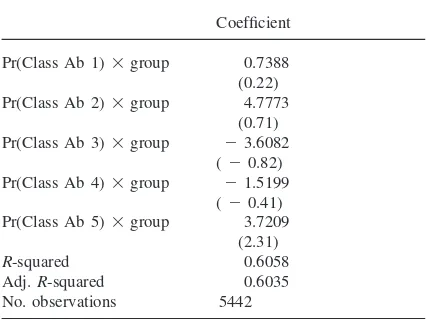
Table 7 compares test scores based on the probability of being in a particular ability group. Only the top stu-dents are significantly affected (positive coefficient). In other words, after instrumenting for the probability of being in a particular class ability level, the difference among the ability levels is reduced to zero for all but level 5 classes. Note also that the range of predicted effects of grouping across ability levels is much more
Table 7
Instrumental variable results for regressions of test scores on interaction of probability of placement in class ability levelsa and grouping
Coefficient Pr(Class Ab 1)3group 0.7388 (0.22) Pr(Class Ab 2)3group 4.7773
(0.71) Pr(Class Ab 3)3group 23.6082
(20.82) Pr(Class Ab 4)3group 21.5199
(20.41) Pr(Class Ab 5)3group 3.7209
(2.31)
R-squared 0.6058
Adj.R-squared 0.6035
No. observations 5442
aClass ability level is determined by the teacher (55highest). Hetero-robustt-statistics in parentheses. Heterogeneous group is the comparison group.
Other regressors included but not shown: lagged test scores, school inputs, school size, percent Hispanic, dummies for grade level, race, sex, region, parents’ education levels, and whether the school is suburban or rural. See the data section for a more detailed description.
modest than in the OLS version of this equation (model 2 in Table 3). The size of the gap in predicted test scores between students in the top and bottom classes in grouped schools is also much closer to what we obtained in models 3–7 in Table 3, where we used control groups of students in classes of similar ability in non-grouped schools.
4.3. Resource allocation
An interesting finding from the above section is that the measured effect of grouping did not change much when we estimated the reduced form models that excluded classroom characteristics. This finding is sur-prising: the theoretical case for grouping rests in part on the notion that once students are grouped by initial achievement, the school can tailor class size and the type of teacher to the needs of the given class. By removing the possibly endogenous measures of school inputs from the regression, the coefficient on the grouping variable should rise to reflect the total effect of grouping, includ-ing the efficiency effects that should result when schools reallocate resources among ability groups. The finding that the coefficient on grouping did not change much when classroom inputs were removed suggests that per-haps schools with formal grouping policies do not in fact reallocate school resources relative to schools without formal grouping. In this section we examine the extent to which formal grouping leads to differences in resource allocation.
If students of differing ability levels benefit from inputs differently, as found by Summers and Wolfe (1977), then schools should be able to reallocate resources in a way that increases test scores of both high and low ability students.14 If schools do not reallocate
resources, they may not be taking advantage of potential efficiency effects.
A second motivation for studying resource allocation within both types of schools derives from the work of Oakes (1990). Oakes argues that grouping leads to a resource allocation that does not benefit all students, but one that favours the top students and top classes. A com-parison of resource allocation in the two types of schools will determine whether grouping schools are exploiting these possibilities, and whether it is done in a way that will increase test scores or increase inequality. To the best of our knowledge, this is the first test of this hypoth-esis using a large nationally representative data set.
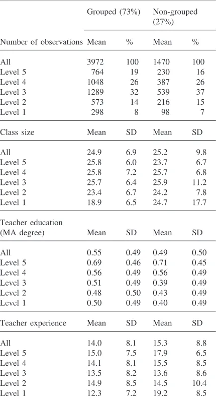
Table 8 lists means of school inputs by class ability level. If non-grouping schools have heterogeneous classes, the non-grouping schools should be relatively clustered around the average ability group, and the grouping schools more spread out among ability levels, but the dispersion is remarkably similar in the two school types.
The claim that grouping causes lower ability students to receive fewer inputs does not fit these data. With respect to class size, the lower ability students in grouped schools actually have a smaller average class size, less than 19, while all other groups are clustered around 25 students per class (special education students, who have smaller classes, are not included in the LSAY data set). In this sample, 69% of high ability students at schools with grouping have teachers with master’s degrees, com-pared to 50% for the grouped classes of lowest ability. But, we find an even greater discrepancy in the schools without ability grouping: 71% in the high classes to 40% in the low classes. Conceivably, the disparity is not caused by grouping, but by the fact that upper level high school math classes require more highly educated teach-ers.
Teacher experience shows the most variation between school types. On average, students at schools with ability grouping have teachers with 1.3 years more experience than those at non-grouping schools. In the schools with-out ability grouping, the lowest ability classes have the most experienced teachers, with an average of 19.2 years of teaching experience. In contrast, of the five grouped levels, the lowest ability group has teachers with the least experience, an average of 12.3 years. This is not neces-sarily deleterious to these students, since evidence exists that lower ability students are particularly helped by less
classes, while high achieving students do better. High achieving students benefit from more experienced teachers, whereas low achieving students are negatively affected, i.e. they benefit more from less experienced teachers.
Table 8
Means and standard deviations (SD) of school inputs for grouped and non-grouped schools by class ability levela
Grouped (73%) Non-grouped (27%) Number of observations Mean % Mean %
All 3972 100 1470 100
Level 5 764 19 230 16
Level 4 1048 26 387 26
Level 3 1289 32 539 37
Level 2 573 14 216 15
Level 1 298 8 98 7
Class size Mean SD Mean SD
All 24.9 6.9 25.2 9.8
Level 5 25.8 6.0 23.7 6.7
Level 4 25.8 7.2 25.7 6.8
Level 3 25.7 6.4 25.9 11.2
Level 2 23.4 6.7 24.2 7.8
Level 1 18.9 6.5 24.7 17.7
Teacher education
(MA degree) Mean SD Mean SD
All 0.55 0.49 0.49 0.50
Level 5 0.69 0.46 0.71 0.45
Level 4 0.56 0.49 0.56 0.49
Level 3 0.51 0.49 0.39 0.49
Level 2 0.48 0.50 0.43 0.49
Level 1 0.50 0.49 0.40 0.49
Teacher experience Mean SD Mean SD
All 14.0 8.1 15.3 8.8
Level 5 15.0 7.5 17.9 6.5
Level 4 14.1 8.1 15.5 8.5
Level 3 13.5 8.2 13.6 8.6
Level 2 14.9 8.5 14.5 10.4
Level 1 12.3 7.2 19.2 8.5
aClass ability level is determined by the teacher (55highest). N55442.
experienced teachers.15,16We repeated this analysis using
achievement quartiles. The #allocation of school inputs across ability levels and between schools with and with-out ability grouping was highly similar to the one in Table 8.17
In sum, it might appear that grouping leads to inequality in resource allocation when comparing inputs among class ability levels only for schools with ability
grouping. But comparisons between schools with and without grouping do not provide compelling evidence for inequality and discrimination due to a formal ability grouping policy.
The above results present means across schools and do not rule out the possibility that grouping increases inequality of resource allocation within a particular school. To test the hypothesis that grouping aggravates inequality in resource allocation within schools, we run panel regressions of classroom resources with fixed effects for individual schools to test for the effect of class ability Eq. (4a) and the effect of relative test score Eq. (4b):
Xit5f(Fi,Cit,Cit3Tit) (4a)
Xit5f(Fi,Sit21/Sigt21,(Sit21/Sigt21)3Tit). (4b)
Here, Sit−1/Sigt−1 is a student’s relative test score. A
positive coefficient on this variable indicates that high achieving students receive more of this input than do low achieving students in the same school. Average class ability level, Cit, is 1–5, where 5 is the highest class
ability. If the coefficient on Cit is positive, then an
increase in class ability levelat a given schoolis associa-ted with an increase in the input being studied. The above examination of means for each input by class ability level suggests that there are differences among resources for class ability levels, meaning that this coef-ficient will be significant for each of the three inputs. This applies to both grouped and non-grouped schools. In order to determine whether a particular school with grouping has even greater differences among class ability levels, the equations contains interaction terms for class ability level and grouping,Cit3Tit, Eq. (4a), and
for relative test score and grouping, (Sit21/Sigt21)3 Tit Eq. (4b). If grouping schools allocate resources to
classes differently based on class or student ability, then the coefficients on one or both of these terms will be sig-nificant.
16We tested this finding by dropping teacher experience and its square from model #1 in Table 3, and including four interac-tion terms for teacher experience and ability quartile, and find a positive (0.065) and significant (p-value50.001) coefficient for the top quartile only. The coefficients for the second, third, and fourth quartiles are negative, withp-values of 0.082, 0.003, and 0.153 respectively. From this evidence, we conclude that students with higher initial test scores benefit from more experi-enced teachers, while those with lower initial scores benefit from less experienced teachers. These results concur with those of Summers and Wolfe (1977).
17The results are available from the authors upon request.
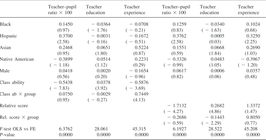
In Table 9, for the first input, teacher–pupil ratio, the coefficients on relative test score and class ability are both negative, indicating that higher ability students are more likely to be put into classes with smaller teacher– pupil ratios, i.e. larger classes. But, the coefficients on the interaction terms are both insignificant, indicating that the teacher–pupil ratio is determined similarly in grouping and non-grouping schools.
We estimate a linear probability model for teacher education. Relative test score and class ability level both have positive and significant effects on the likelihood that a student will be taught by a teacher holding a mas-ter’s degree. In addition, the coefficient on the interaction term for relative test score and grouping is negative and significant, indicating that although higher ability stu-dents are more likely to receive more educated teachers, grouping mitigates this effect. The coefficient on relative test score is 0.27 for non-grouping schools, while for grouping schools it is 0.2720.1450.13, still positive but smaller. The regression using class ability yields a negative but insignificant sign.
This is not the case for teacher experience; students in lower ability classes are likely to have more experienced teachers in non-grouping schools, as evidenced by the negative and significant coefficient ( 2 0.59) on class ability, whereas in grouping schools, students in lower ability classes get less experienced teachers, since the coefficient on the interaction term is positive and sig-nificant. Moving up a class ability level in a grouping school is associated with an increase in teacher experi-ence of2 0.59 1 0.745 0.15, less than a fifth of a year. So compared to higher ability classes, lower ability classes are taught by less experienced teachers in grouped schools, the only indication that grouping causes inequality in resource allocation within schools. More-over, the final column of Table 9 finds that grouping schools do not allocate teachers significantly differently across students of different abilities. Overall, the results do not suggest that the use of formal grouping generates inequality in the distribution of resources. The findings help to explain why test score regressions which excluded possibly endogenous classroom inputs changed the results so little.
5. Conclusion
com-Table 9
Fixed effects regressions for school inputs by school
Teacher–pupil Teacher Teacher Teacher–pupil Teacher Teacher ratio3100 education experience ratio3100 education experience
Black 0.1450 20.0364 20.0708 0.1259 20.0340 0.1024
(0.97) (21.76) (20.21) (0.83) (21.63) (0.68)
Hispanic 0.3700 20.0031 20.1672 0.3762 0.0005 0.3250
(2.58) (20.16) (20.51) (2.58) (0.03) (2.25)
Asian 0.2468 0.0651 0.5224 0.1551 0.0668 0.2690
(0.95) (1.80) (0.87) (0.59) (1.84) (1.03)
Native American 20.3899 0.0514 0.2231 20.3326 0.0483 20.3967
(21.18) (1.12) (0.29) (20.99) (1.05) (21.20)
Male 0.0418 0.0020 20.1654 0.0617 0.0006 0.0357
(0.56) (0.20) (20.96) (0.82) (0.06) (0.48)
Class ability 20.5438 0.0378 20.5876
(27.83) (3.92) (23.69)
Class ab3group 0.0750 20.0029 0.7449
(0.95) (20.27) (4.13)
Relative score 21.7132 0.2682 1.3372
(24.27) (4.86) (1.47)
Rel. score3group 20.2686 20.1443 0.8050
(20.59) (22.29) (0.77)
F-test OLS vs FE 6.3762 28.061 45.315 6.1927 28.522 45.208
P-value 0.0000 0.0000 0.0000 0.0000 0.0000 0.0000
t-statistics in parentheses. Number of schools584.N55442.
Other regressors included but not shown: dummies for grade level and parents’ education levels.
pared to students at schools without grouping. We argue that to some extent these results may be found due to a comparison of high and low ability students to the aver-age ungrouped students. It appears likely that if the model does not control perfectly for the student’s initial achievement, then the coefficients on the class ability proxies will be biased away from zero because they are correlated with the student’s own imperfectly measured ability or motivation. We control for average class ability at not only the grouping schools, but the non-grouping schools as well, using two different measures of class ability and find no significant effects of grouping on the bottom class ability groups. However, we do find some evidence that middle students are harmed by grouping and that the top students are helped, but by less than predicted by the former specification.
We also calculate propensity scores for group place-ment of students and group students into quartiles based on these scores. This allows us to compare students of similar backgrounds and likelihoods of being placed in a particular group. When we run OLS regressions on each of the four propensity quartiles, we find the group-ing variable to be insignificantly different from zero. An approach that uses instrumental variables for class ability level indicates significant effects of grouping only on the highest level classes. Previous evidence for the differen-tial effects of grouping may in part reflect inadequate
controls for class ability level at the non-grouping school.
In addition, at least some of the blame for inequality in student achievement and class resources may have been erroneously ascribed to ability grouping. Using panel regressions with fixed effects for schools, we show that both types of schools allocate smaller classes to the lower ability students and that ability grouping does not increase or diminish this effect. The results for teacher education indicate that both types of school are more likely to allocate teachers with master’s degrees to higher ability students and classes. Moreover, schools with for-mal ability grouping policies seem to mitigate the inequality. In the case of teacher experience, higher achieving students in the grouped schools are more likely to be taught by more experienced teachers than their lower achieving counterparts, and vice versa for non-grouped students. This can be viewed as evidence that grouping generates inequality. But if, as some research shows, lower ability students benefit more from less experienced teachers, then it can be interpreted as an increase in efficiency.
policies on student achievement. Second, it reproduces the results found in previous studies, that grouping leads to large differential effects, and argues that these results may in part reflect inadequate control groups. Although the paper does find some evidence that grouping has dif-ferential effects across students of differing ability levels, after controlling for class ability level in the non-group-ing schools, the sizes of the effects are shown to be far smaller than previous estimates. Third, there is little evi-dence that ability grouping generates inequality in the allocation of school resources among classes. This does not mean that ability grouping is necessarily ineffectual. One possible interpretation of these results is that all schools group students to some extent, even if there is no formal grouping policy.
Acknowledgements
This research was supported by a Dissertation Grant to Shkolnik from the American Educational Research Association, which receives funds for its ‘AERA Grants Program’ from the National Science Foundation and the National Center for Education Statistics (U.S. Depart-ment of Education) under NSF Grant #RED-9452861. Opinions reflect those of the authors and do not necessar-ily reflect those of the granting agencies.
References
Alexander, K. L., & Cook, M. A. (1982). Curricula and course-work: a surprise ending to a familiar story.American Socio-logical Review,47, 626–640.
Alexander, K. L., & McDill, E. L. (1976). Selection and allo-cation within schools: some causes and consequences of cur-riculum placement. American Sociological Review, 41, 963–980.
Argys, L. M., Rees, D. I., & Brewer, D. J. (1996). Detracking
America’s schools: equity at zero cost?Journal of Policy Analysis and Management,15(4), 623–645.
Bowden, R. J., & Turkington, D. A. (1984).Instrumental vari-ables. Cambridge: Cambridge University Press.
Gamoran, A. (1987). The stratification of high school learning opportunities.Sociology of Education,60, 135–155. Gamoran, A., & Berends, M. (1987). The effects of
stratifi-cation in secondary schools: synthesis of survey and ethno-graphic research. Review of Educational Research, 57, 415–435.
Greene, W. H. (1993).Econometric analysis. New York: Mac-millan.
Hallinan, M. (1990). The effects of ability grouping in second-ary schools: a response to Slavin’s best-evidence synthesis. Review of Educational Research,60, 501–504.
Hoffer, T. B. (1992). Middle school ability grouping and stud-ent achievemstud-ent in science and mathematics. Educational Evaluation and Policy Analysis,14, 205–227.
Jencks, C. S., & Brown, M. D. (1975). Effects of high schools on their students.Harvard Educational Review, 45, 273– 324.
Kerckhoff, A. C. (1986). Effects of ability grouping in British secondary schools. American Sociological Review, 51, 842–858.
Miller, J. D., Hoffer, T., Suchner, R. W., Brown, K. G., & Nelson, C. (1992). LSAY codebook: student, parent, and teacher data for cohort one for longitudinal years one through four (1987–1991). DeKalb, Illinois: Northern Illi-nois University.
Oakes, J. (1990).Multiplying inequalities—the effects of race, social class, and tracking on opportunities to learn math-ematics and science. Santa Monica: RAND.
Rosenbaum, P., & Rubin, D. (1983). The central role of the propensity score in observational studies for causal effects. Biometrika,70, 41–55.
Slavin, R. (1990). The effects of ability grouping in secondary schools: a best-evidence synthesis.Review of Educational Research,60, 471–499.