Review
Bases and limits to using ‘degree.day’ units
Raymond Bonhomme *
INRA Unite´ de Recherche en Bioclimatologie,78850 Thi6er6al-Grignon, France
Received 10 August 1999; received in revised form 3 February 2000; accepted 4 April 2000
Abstract
Degree.day units, for which there are also several synonymous terms, are often used in agronomy essentially to estimate or predict the lengths of the different phases of development. The physiological and mathematical bases upon which they are founded are, however, sometimes forgotten, resulting in questionable interpretations. Such is particularly the case for anything relating to variations in the temperature thresholds which enter into the calculation of these degree.day sums. Without seeking to draw up a synthesis of the extremely numerous works published in the field, this review article sets out to present the basic principles of the degree.day unit notion as well as the limits of its use. On this last point, we will particularly emphasise the influence of the non-linearity of the temperature response of the method used in determining the threshold temperature as well as the pertinence of the temperature taken into account in studying the phenomenon. Several practical conclusions are drawn from this review article. © 2000 Elsevier Science B.V. All rights reserved.
Keywords:Base temperature; Day-degrees; Growing degree-days; Heat sums; Heat units; Thermal time; Thermal units; Threshold temperature
www.elsevier.com/locate/eja
1. Introduction
The effects of temperature on physiological phenomena are numerous. For example, in John-son and Thornley (1985) one finds an attempt at developing a conceptual outline of the different action laws both at the level of the various
chem-ical reactions (Arrhenius’ equation, Q10 factor,
reactions with or without optimum temperature) or phenomena such as diffusion, viscosity and translocations, and at the level of the organ, the plant or the cultivation: effect of temperature on
photosynthesis, respiration or rate of
development.
In general, the effect of temperatures on plant functioning is brought about by the action on enzymatic activities. The conformation of en-zymes is the essential step in the enzymatic
reac-tion and this conformation depends on
temperature. At too low a temperature the
en-* Tel.: +33-130-815555; fax:+33-130-815563.
E-mail address: [email protected] (R. Bon-homme)
zyme protein is not flexible enough and therefore not in a position to carry out the conformation change required for the reaction; at too high a temperature the enzyme coagulates and the new structure thus obtained is not able to catalyze the reaction. Temperature action curves thus typically have two sides: a growth segment where thermal activation of the molecules increases the efficiency of the reactions and a diminishing segment where the high temperatures progressively inactivate cer-tain enzymes. Between these two sides the curve reaches a peak corresponding to the optimal tem-perature (Bourdu, 1984). It is for this reason that we have a minimum, a maximum, and an opti-mum temperature for the temperature responses.
A large number of enzymes play a role in plant development and presumably enzymes providing photosynthates are very important. There is a great deal of difference between C-3 and C-4 species as far as the enzymes involved in photo-synthate production are concerned. The pyruvate-phosphate dikinase, which provides the PEP and
hence the CO2acceptor in C-4 species, is sensitive
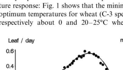
to low temperatures (Edwards, 1986) whereas the Rubisco found in the C-3 species is very efficient even at low temperatures. This difference is clearly expressed in the leaf development tempera-ture response: Fig. 1 shows that the minimum and optimum temperatures for wheat (C-3 species) are respectively about 0 and 20 – 25°C whereas for
maize (C-4 species) they are respectively about 10 and 30 – 35°C.
The ‘degree-day’ unit stems mainly from the relationship between development rate and tem-perature. It was Re´aumur (1735) who first laid the basis of this notion: ‘The same grains are har-vested in very different climates; it would be interesting to compare the sums of heat degrees over the months during which wheat does most of its growing and reaches complete maturity in hot countries, like Spain or Africa … in temperate countries, like France … and in the colder coun-tries of the North,’ (original text in Old French: Durand, 1969). Even if the exact vocabulary was not correct (what is a sum of heat degrees?), the concept of a relationship between the develop-ment rate of crops (here the sowing to maturity period) and temperature was born.
Hundreds of works have set about using, prov-ing, or even disproving this idea. Several com-ments can be made:
We will limit ourselves to works on develop-ment rate, with ‘developdevelop-ment’ taken in the sense of ‘the series of identifiable events resulting in a qualitative (germination, flowering, etc.) or quan-titative (number of leaves, flowers, etc.) modifica-tion of plant structure.’ The relamodifica-tionships between growth rate and temperature have, however, also been the object of numerous studies: the most often quoted experimental result in studies dealing with the effect of temperature on plants is cer-tainly the action law concerning the effect of temperature on the growth in length of maize coleoptiles (Lehenbauer, 1914). It is true that separating growth phenomena from developmen-tal phenomena is a bit artificial, as the two are connected (for example, growth often implies the appearance of specific new tissues; Rageau, 1985). Moreover, it is interesting to note the similarity between the form of the temperature response for a developmental phenomenon (rate of leaf emer-gence, Tollenaar et al., 1979; Fig. 1: curve) and for a growth phenomenon (coleoptile elongation, Lehenbauer, 1914; Fig. 1: dots). This similarity is all the more noticeable when the maize genotypes change a lot between the two periods. It should be noted that the rate of leaf emergence is the inverse of the duration separating the appearance of two
successive leaves, a period sometimes called ‘phyllochron’
From the moment that interest was turned to working on spring crops, which develop only under largely positive temperature conditions, or
to using the Fahrenheit temperature scale (0°C=
32 F) it became necessary to introduce the threshold temperature concept (below which the rate of development is considered to be nil).
Methods for determining this temperature
threshold (to give a good prediction of a specific phase) as well as research into differences between species or between plants of a same species have given a large number of works.
It has often been found that the linearity be-tween development rate and temperature is only valuable for a relatively limited range of tempera-tures. For example, the experimental curve in Fig. 1 shows that:
• Near threshold temperature the relationship is practically exponential, an observation
explain-ing the use of Q10 sums within this range
(Bidabe´, 1967; Niqueux and Arnaud, 1967). • The action law peaks then rapidly decreases.
Determining the last part of this curve experi-mentally remains, however, very difficult due to the inevitable interactions with water stress at high temperatures. Even if the maximum position varies greatly between species and genotypes, there are very few biological phe-nomena occurring above 45°C.
2. Rate and path of development
If one considers:
• A time spanDt=1 day
• That development rate, R, is proportional to
the daily temperature, Td, reduced by a
threshold temperature,Tt, then:R=a(Td−Tt)
this same daily growth rateRis the inverse of the
total duration, in days, of the phase (for example, from sowing to flowering, from the emergence of
leaf n to that of leaf n+1, etc.), so:
The path of development (rate×time) for one
day is, therefore:
and the total path of development for the phase:
%
degree.day sum which is, therefore, a constant equal to 1/a.
To represent the example given in Fig. 1 in numerical form, by linearizing for the 10 – 30°C interval, the temperature response of the foliar appearance, one obtains approximately:
R=a(Td−10) with a=0.033
with R in d−1
and a in (degree.day)−1
. The fraction of development path obtained during 1
day with a temperature Td=25°C is 0.5 (at this
constant temperature the development of one leaf
in 1/0.5=2 days). Should T=13°C, the fraction
of development path becomes 0.1 (a leaf appears in 10 days). The total path of development for the
appearance of a leaf in degree.day is 1/a, hence 30
degree.day. Therefore, a 25°C day results in a sum
of (25−10)=15 degree.day (thus, at constant
temperature, a leaf appears in 30/15=2 days). At
13°C days the resulting leaf appearance in 30/
(13−10)=10 days.
3. Examples of the use of degree.day units
The practical impact of using degree.day sums is considerable (Ritchie and NeSmith, 1991). To mention but a few examples, they can be used to: • Classify plants for their flowering rate or length
of cycle (Derieux and Bonhomme, 1982a,b).
• Estimate harvest maturity (Gilmore and
• Schedule vegetable harvesting according to their level of tenderness (Katz, 1946, for peas). • Predict the duration, under natural conditions, between two developmental stages for a para-site used in biological control (Bernal and Gonzalez, 1993).
• Anticipate insect development with a view to better phytosanitary control (Pruess, 1983). • Assess sporulation intensity for a cereal fungus
(Tyldesley, 1978), etc.
Still, this profusion of works using degree.day units sometimes results in the bases of the method being forgotten:
• Linearity between growing rate and
temperature.
• Unequivocal relationship between growth rate and temperature.
• Obvious representational quality of tempera-ture taken as a reference in relationship to the studied phenomenon.
• Absence of any other factor limiting
development.
These different points will now be discussed.
4. Influence of non-linearity between development rate and temperature
Fig. 1 clearly shows that development rate can be considered as linearly proportional to tempera-ture for only a short range of temperatempera-ture varia-tion. Using present-day calculation tools it is perfectly possible to calculate growth over a daily or even shorter time span using a more or less complicated development rate law. As examples taken from the case of maize (Bonhomme et al., 1994), let us cite a few non-linear methods used to estimate the daily development DD (always posi-tive or nil), in function of minimum daily
temper-ature, Tn, and maximum daily temperature, Tx:
DD=(Q10)
(T/10), with Q
10 values close to 2
DD=0.0997−0.0360T+0.00362T2
−0.0000639T3
,
according to Tollenaar et al. (1979)
DD= −2.80+0.59T−0.046T2+0.0019T3
−0.000027T4,
according to Blacklow (1972).In these three
for-mulae DD equals the average obtained usingT=
Tn and T=Tx.
DD=0.5[3.33(Tx−10)−0.084(Tx−10)
2
+1.85(Tn−4.4)],
Ontario Corn Unit Method (Brown, 1975). The increased calculation complexity brought about by using these formulae often results in quite minor improvements in the prediction of phase length (Bonhomme et al., 1994). It is, there-fore, common to keep the simple calculation of development in degree.day sums while taking into account the fact that non-linearity will have sev-eral types of influence:
4.1. Depending on the temperature range at which linearization is carried out
An initial graphical estimate as to this effect can be seen in Fig. 1. Under relatively low tem-perature conditions the temtem-perature threshold es-timated by linearization of the curve over a specific range of temperatures will be lower than that estimated over warmer situations. Here one finds the explanation to the polemic concerning the superiority of the ‘French method’ of calculat-ing degree.day sums (with 6 – 7°C temperature thresholds; Bloc and Gouet, 1977) over the ‘American methods’ (with temperature thresholds around 10°C). The difference lies simply in the fact that maize cultivation temperatures are, on an average, higher in the USA than in France!
Sinclair (1994) gives an analytical presentation of this effect for temperatures quite close to threshold level. A system’s reaction rate can, hence, be described by a temperature exponential function (Arrhenius’ equation):
R=Bexp(−A/CT)
where A is the system’s activation energy (J
mol−1
), Cthe gas constant (8.31 J mol−1
K−1
),
Tthe temperature (K) andBa constant. Reaction
rate can be presented in correspondence to a
reference temperature, Tref:
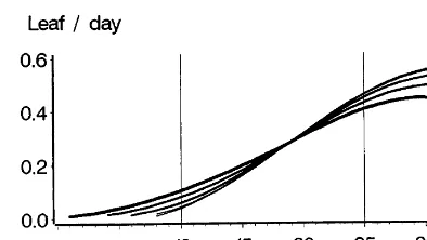
Fig. 2. Fine line: corn leaf appearance rate as a function of temperature (according to Tollenaar et al., 1979). The curves with progressively thicker lines show the deformation of this action law if the temperature under question is the average daily temperature and if it is assumed that the daily tempera-ture variation is a sinusoidal form with an increasing ampli-tude (as with the thickness of the lines: 5, 10, 15 and 20°C).
those in Cao and Moss (1991), affirming that degree.day needs are higher for the final leaves than for the first leaves to appear, can only be accepted with a certain amount of precaution.
4.2. Depending on daily thermal amplitude
Throughout the day, actual temperatures vary around the daily average temperature according to an approximately sinusoidal curve. The result of this situation is that even if the daily average
temperature equals the temperature threshold Tt
(one should find a daily development of zero if the
daily temperature remains equal to Tt), there is a
certain amount of development due to the daily period during which the actual temperatures rise above Tt.
Fig. 2 shows daily growth on days of given temperatures and thermal amplitudes, assuming sinusoidal variation in daily temperatures. It was developed according to the development rate law as a function of temperature given in Tollenaar et al. (1979). The results of a linear treatment of the different curves in the 10 – 25°C range are shown in Table 1. It is apparent that threshold tempera-ture drops with the increase of the daily thermal amplitude.
5. Influence of the method used in determining the action law
The value of the estimated threshold tempera-ture also depends on the method used in deter-mining it. Even though they have been used by certain authors, methods drawing upon relations between variables cumulated in time (for example, degree.day sum and the number of leaves which appeared) should be avoided (Malet et al., 1997). Different types of information are sought by different authors. They can be outlined as: Since biological phenomena take place within
quite limited ranges of temperature, Tref can be
taken from the middle of this range; one can then
limit the margin of error by replacing T.Tref by
Tref2 . Moreover, A/(C.Tref2 ) is small and one can
linearize the exponential:
R/Rref:1+
A CTref2
(T−Tref)
What one usually seeks to do is to extrapolate this slope so as to find the temperature threshold,
Tt, for which the development rate is nil (R/Rref=
0), in which case one has:
Tt=Tref(1−CTref/A)
The temperature threshold Tt which is
esti-mated depends on the reference temperature around which one carries out linearization of the
exponential law. Since (CTref/A) is small, the
higher the Tref, the larger the value of Tt. It is,
therefore, only possible to compare Tt between
experiments, species or plants if the thermal con-ditions are similar. For example, results such as
Table 1
Apparent variation in the threshold temperatureTtobtained by linearization in the 10–20°C interval of the different development laws of Fig. 2 obtained for various daily thermal amplitudes
10 5
0
Daily thermal amplitude (°C) 15 20
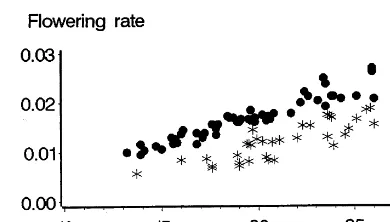
Fig. 3. Relationships between flowering rates (the inverse of sowing – flowering duration in days) and the mean temperature for the period for: an early genotype of temperate origin, LG11 (points), a late genotype of tropical origin, X304C (stars), for a set of trials in numerous countries and under conditions without stresses (Bonhomme et al., 1994).
• The coefficient of variation of the differences between predicted and observed dates (M3). • The regression between the degree.day sums
and the mean temperatures for the different trials (M4), finding the independence between the degree.day sums and the temperatures of the trials.
It should be noted that:
• Differences in development date estimations remain limited when the estimated temperature
is only slightly lower than the real Tt value,
whereas they quickly expand if too high a Tt
value is used (Durand et al., 1982).
• These methods require running a large number
of calculations with different possible Tt
tem-perature thresholds. To avoid these iterative calculations Yang et al. (1995) developed math-ematical formulae which make a direct
calcula-tion of Tt possible. For example, the
temperature threshold Tt which minimizes the
variation coefficient (M3) is:
Tt=
whereTiis the average temperature over the total
duration of the stage under study in trial i, dithe
duration of this stage in days andnthe number of
trials.
If one wishes to display inter- or intra-species differences in the action laws of temperature on development to select, for example, maize capable of being planted earlier and, therefore, at lower temperatures (Giauffret et al., 1995), the compari-sons must be based on the abscissa at the origin and on the slope of the curve relating the relation-ship between development rate and temperature (M5). Whenever one makes a regression between couples (development rate, that is the inverse of
the duration of the stage)×(mean temperature
during the stage) which are available over the different trials, each of the variables is flawed by error. It is therefore preferable to carry out an orthogonal regression (Dagne´lie, 1973).
The sowing-flowering rates for genotype LG11 displayed in Fig. 3 (points), lead to different
temperature threshold valuesTt depending on the
Table 2
Estimation of the threshold temperatureTt obtained for the sowing–flowering rate of LG11 genotype (points in Fig. 3) or X304C genotype (stars in Fig. 3) using various methods (Mx, see text) for determining the development law.
M4
• Either one seeks the temperature threshold which will give the best prediction of the devel-opmental stage using the degree.day sums. • Or one strives to display differences between
species or genotypes in development rates de-pending on the temperature (for example, flow-ering or maturation, leaf appearance rate). The temperature threshold has only statistical value, often quite distant from the ‘physiological temperature’ for which development is zero. In particular, the temperature thresholds which pro-duce the best predictions for a given development stage are usually quite low and depend upon the statistical estimation methods used (Durand et al., 1982). The methods most often used are those
seeking the Tt temperature which minimizes:
• The standard deviation in degree.day sums for a series of trials (M1).
method of estimation (Table 2). Such a result explains the large number of more or less contra-dictory publications relative to determining tem-perature thresholds. It appears quite obvious that
it is just a case of temperatures with
merely statistical value, since at temperatures be-low approximately 10°C there is no growth in maize.
6. Influence of the representational quality of the reference temperature used
It is the temperature of the developing organ which should serve to establish the action law for the phenomenon under study and, therefore, cal-culation of degree.day sums. Such is practically never possible, but one must still remain vigilant as to:
• The quality of measuring devices: drift, even slow, can have a large cumulative effect. • The fact that the site at which temperatures are
measured must be very near the site where the observations or the growth estimates are made, with particular attention being paid to the ef-fects of different expositions or altitudes. • The estimation of mean temperature on the
basis of minimum and maximum daily temper-atures, an approximation which is susceptible of provoking a divergence (slight over-estimate for mean photoperiods and under-estimate for short and long photoperiods; Hallaire, 1950). • The position of the ‘sensitive plant organ’: for
example, maize leaf emergence rate will be more closely linked to ground temperature for the first foliar stages because the apex is then at the surface of the ground, whereas subsequent leaf emergence rates will be more closely linked to air temperature (Duburcq et al., 1983; Swan et al., 1987). For spring sowings, ground tem-perature is always higher than air temtem-perature, which can lead, especially for temperature around threshold level, to wide-scale diver-gence in the calculations of degree.day sums (Ritchie and NeSmith, 1991).
Development of relatively simple models of the energetic balance of plant organs such as the apex (Cellier et al., 1993), the zone of leaf production,
should be continued in order to replace meteoro-logical temperatures by explicative temperatures more pertinent at the level of plant development. To witness, the work of Jamieson et al. (1995) in which it is shown that the affirmations of certain authors as to variations in wheat phyllochrone on the basis of foliar rank or photoperiod are the result of having used bad reference temperatures.
These variations are greatly reduced when
one first refers to ground temperature and later to plant temperature after a certain stage in growth.
7. Influence of other factors modifying development rate
The values corresponding to genotype X304C on Fig. 3 (stars) show that sowing-flowering rates are, at the same temperature, lower than for genotype LG11. This means simply that genotype X304C will flower later (that is to say, it has a higher degree.day sum).
If one seeks the temperature thresholds which would make better flowering prediction possible using degree.day sums, one finds that they are higher than for genotype LG11 (Table 2).
Since the X304C is a genotype of tropical origin, one could be led to believe that it is a question of physiological adaptation to higher temperatures than for the LG11, of French origin. In fact, one must first of all note the more marked development rate dispersion, which can be charac-terized by the fact that the quadratic mean error for the regression between growth rate and tem-perature, is 0.0014 for LG11 and 0.0020 for X304C. Fig. 3 shows a high dispersion of points at low and mean temperatures, which is due to the fact that this genotype is a ‘short day’ genotype (Bonhomme et al., 1994) and that, therefore, for long photoperiods development rates, at a given temperature, can be reduced by this photoperiodic sensitivity (Brisson and Dele´colle, 1991).
If one assumes that:
• For a day longer than 13 h, there is no interac-tion between temperature acinterac-tion and photo
period, P, action (Roberts and Summerfield,
1987: R=a%(Td−Tt)+b%(P−13)).
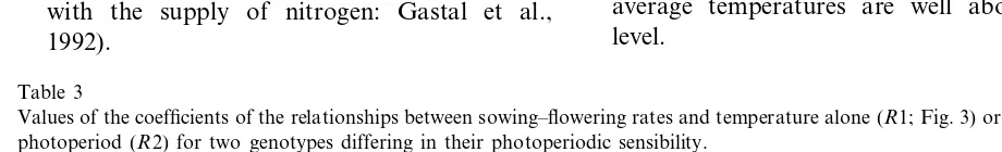
one obtains the results shown in Table 3 for the Fig. 3 data.
It thus becomes obvious that if one takes the photoperiodic sensitivity of genotype X304C into
account, its estimated threshold temperatureTt is
very close to that of LG11. For this ‘short day’ plant, the apparent temperature threshold is in-creased by the long photoperiod.
It is, therefore, very important to take the possible influence of other environmental factors into account when comparing laws concerning the action of temperature on crop growth. It is thus that:
• Photoperiodic effects can be interpreted as ver-nalization effects on ‘long day’ plants, because the estimated temperature threshold can be very low for long days while photoperiodic
thresholds are low (Summerfield et al.,
1989).
• Water stress can accelerate or depress the de-velopment rate depending upon the importance of stress (Brisson and Dele´colle, 1991). With this constraint the temperature of the plant can be considerably different from that of the air and it can be interesting to measure it so as to better estimate development stages (Casals, 1996); a ‘stress degree.day’ approach using canopy temperature can be used (Idso et al., 1978).
• The nutritional state of the plant can have an effect on development phenomena (the leaf emergence temperature response slightly varies with the supply of nitrogen: Gastal et al., 1992).
8. Practical conclusions
The term ‘heat sums’ has no physical reality and it is preferable to use the terms ‘thermal time’
or ‘progress towards …x stage.’
It is of no meaning in giving a degree.day sum without the temperature threshold used for calcu-lating it.
Phyllochron is the time duration, usually given in days, which separates the appearance of two successive leaves; phyllotherm is the correspond-ing degree.day sum; plastochron is the time dura-tion, in days, which separates the initiation of two successive leaves.
It is preferable not to use degree.day sums for the study of growth phenomena without previous reflection about the meaning and definition of
growth (kg m−2 degree.day−1). Among others,
‘Monteith type’ growth analysis (Monteith, 1977; Varlet Grancher, 1982) makes it possible to clearly separate the duration of a stage (evaluated using degree.day sums) from the production of biomass during the same stage because its first approximation is linked to the duration in days, if there is not too much variation in solar radiation and foliar development.
Determining the temperature threshold is only possible if one disposes of development rates obtained for wide ranges in temperature var-iation and in the absence of other eventual limits to growth rate (non-optimal photoperiod, non-vernalization, water or nutritional stress, etc.).
The temperature threshold has only a slight influence on the precision in determining a stage if average temperatures are well above threshold level.
Table 3
Values of the coefficients of the relationships between sowing–flowering rates and temperature alone (R1; Fig. 3) or temperature and photoperiod (R2) for two genotypes differing in their photoperiodic sensibility.
R1=a(Td−Tt)
Genotype R2=a%(Td−Tt)+b(P−13)
Tt
a a% B Tt
LG11 0.00112 4.520 0.00112 0 4.520
One must always try to measure or estimate the temperature of the developing organ even in greenhouses and growth chambers.
It is now perfectly possible to work with tem-perature action laws which are non-linear or with short time intervals (taking diurnal temperature variation into account), but one must first be sure whether this is really worth the effort because one losses statistical power of linear models when one uses such linear laws. If one uses these non-linear models, it is best to use the relatively ‘flex-ible’ mathematical laws with few parameters (for example, Beta laws: Yin et al., 1995).
References
Bernal, J., Gonzalez, D., 1993. Experimental assessment of a degree-day model for predicting the development of para-sites in the field. J. Appl. Ent. 116, 459 – 466.
Bidabe´, B., 1967. Action de la tempe´rature sur l’e´volution des bourgeons de pommiers et comparaison de me´thodes de controˆle de l’e´poque de floraison. Ann. Physiol. Ve´g. 1, 65 – 86.
Blacklow, W.M., 1972. Influence of temperature on germina-tion and elongagermina-tion of the radicle and shoot of corn (Zea maysL.). Crop Sci. 12, 647 – 650.
Bloc, D., Gouet, J.P., 1977. Influence des sommes de tempe´ra-tures sur la floraison et la maturite´ du maı¨s. Ann. Ame´lior. Plant. 28, 89 – 111.
Bonhomme, R., Derieux, M., Edmeades, G.O., 1994. Flower-ing of diverse maize cultivars in relation to temperature and photoperiod in multilocation field trials. Crop Sci. 34, 156 – 164.
Bourdu, R., 1984. Bases physiologiques de l’action des tempe´r-atures. In: Gallais, A. (Ed.), Physiologie du maı¨s. INRA, Paris, pp. 389 – 424.
Brisson, N., Dele´colle, R., 1991. De´veloppement et mode`les de simulation de culture. Agronomie 12, 253 – 263.
Brown, D.M., 1975. Heat units for corn in Southern Ontario. Ontario Ministry of Agriculture and Food, Agdex Fact-sheet 111/31.
Cao, W., Moss, D.N., 1991. Phyllochron change in winter wheat with planting date and environmental changes. Agron. J. 83, 396 – 401.
Casals, M.L., 1996. Introduction des me´canismes de re´sistance a` la se´cheresse du ble´ dur au fonctionnement phe´nologique et trophique de la plante dans un mode`le dynamique de croissance. PhD Thesis INA-PG, Paris, France, 130 pp. Cellier, P., Ruget, F., Bonhomme, R., 1993. Estimating the
temperature of a maize apex during early growth stages. Agric. For. Meteorol. 63, 35 – 54.
Dagne´lie, P., 1973. The´orie et me´thodes statistiques: applica-tions agronomiques. Les Presses Agronomiques de Gem-bloux, Belgique, p. 378.
Derieux, M., Bonhomme, R., 1982a. Heat unit requirements for maize hybrids in Europe: results of the European FAO sub-network. I: sowing – silking period. Maydica XXVII, 59 – 77.
Derieux, M., Bonhomme, R., 1982b. Heat unit requirements for maize hybrids in Europe: results of the European FAO sub-network. II: period from silking to maturity. Maydica XXVII, 79 – 96.
Duburcq, J.B., Bonhomme, R., Derieux, M., 1983. Dure´e des phases ve´ge´tative et reproductrice chez le maı¨s: influence du ge´notype et du milieu. Agronomie 3, 941 – 946. Durand, R., Bonhomme, R., Derieux, M., 1982. Seuil optimal
des sommes de tempe´rature: application au maı¨s (Zea mays
L.). Agronomie 7, 589 – 597.
Durand, R., 1969. Signification et porte´e des sommes de tempe´rature. BTI 238, 185 – 190.
Edwards, G.E., 1986. Carbon fixation and partitioning in the leaf. In: Shannon, J.C., Knievel, D.P., Boyer, C.D. (Eds.), Regulation of carbon and nitrogen reduction and utiliza-tion in maize. Am. Soc. Plant Physiologists, Rockville, MA, pp. 51 – 65.
Gastal, F., Belanger, G., Lemaire, G., 1992. A model of the leaf extension rate of tall fescue in response to nitrogen and temperature. Ann. Bot. 70, 437 – 442.
Giauffret, C., Bonhomme, R., Derieux, M., 1995. Genotypic differences for temperature response of leaf appearance rate and leaf elongation rate in field-grown maize. Agronomie 15, 123 – 137.
Gilmore, E.C., Rogers, J.S., 1958. Heat units as a method of measuring maturity in corn. Agron. J. 50, 611 – 615. Hallaire, M., 1950. Les tempe´ratures moyennes nocturnes,
diurnes et nycthe´me´rales exprime´es en fonction du mini-mum et du maximini-mum journaliers de tempe´rature. C.R. Acad. Sci. 231, 1533 – 1535.
Idso, S.B., Jackson, R.D., Reginato, R.J., 1978. Extending the ‘degree day’ concept of plant phenological development to include water stress effects. Ecology 59, 431 – 433. Jamieson, P.D., Brooking, I.R., Porter, J.R., Wilson, D.R.,
1995. Prediction of leaf appearance in wheat: a question of temperature. Field Crops Res. 41, 35 – 44.
Johnson, I.R., Thornley, J.H.M., 1985. Temperature depen-dence of plant and crop processes. Ann. Bot. 55, 1 – 24. Katz, Y.H., 1946. The relationship between heat unit
accumu-lation and the planting and harvesting of canning peas. Agron. J. 38, 74 – 78.
Lehenbauer, P.A., 1914. Growth of maize seedlings in relation to temperature. Physiol. Res. 5, 247 – 288.
Malet, P., Pe´caut, F., Bruchou, C., 1997. Beware of using cumulated variables in growth and development models. Agric. For. Meteorol 88, 137 – 143.
Monteith, J.L., 1977. Climate and the efficiency of crop pro-duction in Britain. Phil. Trans. R. Soc. London 281B, 277 – 294.
Pruess, K.P., 1983. Day-degree methods for pest management. Environmental Entomology 12, 613 – 619.
Rageau, R., 1985. Phe´nome`ne de croissance: action du climat. In: De´partement de Bioclimatologie (Ed), Les bases de la Bioclimatologie. 2-Bases biologiques. INRA Grignon, France, pp 135 – 167.
Re´aumur, R.A., 1735. Observations du thermome`tre faites pendant l’anne´e MDCCXXXV compare´es a` celles qui ont e´te´ faites sous la ligne a` l’Isle-de-France, a` Alger et en quelques-unes de nos Isles de l’Ame´rique. Me´moires de l’Acade´mie Royale des Sciences, 545-576.
Ritchie, J.T., NeSmith, D.S., 1991. Temperature and crop development. In: Hanks, J., Ritchie, J.T. (Eds.), Modeling plant and soil systems. ASA, USA, pp. 5 – 29.
Roberts, E.H., Summerfield, R.J., 1987. Measurement and prediction of flowering in annual crops. In: Atherton, J.G. (Ed.), Manipulation of Flowering. Butterworths, London, pp. 17 – 50.
Sinclair, T.R., 1994. Limits to crop yield? In: Boote, K.J., Bennett, J.M., Sinclair, T.R., Paulsen, G.M. (Eds.), Physi-ology and determination of crop yield. ASA, USA, pp. 509 – 532.
Summerfield, R.J., Ellis, R.H., Roberts, E.H., 1989. Vernaliza-tion in chickpea (Cicer arietinum): fact or artefact. Ann. Bot. 64, 599 – 603.
Swan, J.B., Schneider, E.C., Moncrief, J.F., Paulson, W.H., Peterson, A.E., 1987. Estimating corn growth, yield and grain moisture from air growing degree days and residue cover. Agron. J. 79, 53 – 60.
Tollenaar, M., Daynard, T.B., Hunter, R.B., 1979. Effect of temperature on rate of leaf appearance and flowering date in maize. Crop Sci. 19, 363 – 366.
Tyldesley, J.B., 1978. A method of evaluating the effect of temperature on an organism when the response is non-lin-ear. Agric. Met. 19, 137 – 153.
Varlet Grancher, C., 1982. Analyse du rendement de la con-version de l’e´nergie solaire par un couvert ve´ge´tal. PhD Thesis, Orsay, France, 144 pp.
Yang, S., Logan, J., Coffey, D.L., 1995. Mathematical formu-lae for calculating the base temperature for growing degree days. Agric. For. Met. 74, 61 – 74.
Yin, X., Kropff, M.J., McLaren, G., Visperas, R.M., 1995. A nonlinear model for crop development as a function of temperature. Agric. For. Met. 77, 1 – 16.