*Corresponding author. Tel.: #45-89-4235-47; fax: 45-86-1317-69.
E-mail address:[email protected] (S.G. Johansen).
The (r,
Q) control of a periodic-review inventory system with
continuous demand and lost sales
S
+
ren Glud Johansen
!
,
*, Roger M. Hill
"
!Department of Operations Research, University of Aarhus, Ny Munkegade, DK-8000 Asrhus C, Denmark
"School of Mathematical Sciences, University of Exeter, Exeter EX4 4QE, UK
Received 6 April 1998; accepted 28 January 2000
Abstract
In this paper we consider a periodic review inventory model with lost sales during a stockout and with the constraint that at most one replenishment order may be outstanding at any time. Demands in successive review periods are independent, identically distributed variables from a continuous distribution. The"xed lead time is an integral number of review periods. We explore control policies of the (r,Q) type}that is a replenishment order of sizeQis placed when the inventory position (stock in hand plus stock on order) falls to or below the re-order levelr. We use asymptotic renewal theory results to estimate the&undershoot'of the re-order levelrand also to estimate the cycle stockholding cost (which turns out to take a relatively simple form). Based on these approximations we set out a policy improvement solution methodology and illustrate this with some numerical examples for which demand is normally distributed. These numerical examples suggest that a relatively simple approach, based on the economic order quantity, can provide results which are very close to optimal. ( 2000 Elsevier Science B.V. All rights reserved.
Keywords: Inventory; Periodic review; Lost sales; Renewal theory; Undershoot
1. Introduction
In this paper we consider a periodic review inventory model with lost sales during a stockout. Demands in successive review periods are indepen-dent, identically distributed variables from a con-tinuous distribution. We explore control policies of the (r,Q) type}that is a replenishment order of size Qis placed when the inventory position (stock in hand plus stock on order) falls to or below the
re-order level r. It is assumed that the optimal policy will be such that there will never be more than one order outstanding at any time, which means thatQ'r. The lead time is"xed and is an integral multiple of the review interval }this last assumption simpli"es the computation of the stockholding cost but it can be relaxed by allowing the review interval and the lead time to be integral multiples of some (small) basic period, such as a working day, as suggested in Janssen et al. [1]. The analysis extends to variable lead time but its practicality then depends on whether or not a closed form exists for the distribution of demand in lead time. Note that for a lost sales formula-tion the optimal control policy will, in general, be
neither of the (r,Q) type nor of the (s,S) type but will depend in a much more complex way on the phys-ical stock at the time of placing an order. The complexity of optimal lost sales control policies contrasts with optimal backorder control policies, which, for this formulation, can be shown to be of the (s,S) type. Note also that, for variable lead time, the computation of the optimal policy is more complicated if the lead time is not unimodal.
In many inventory formulations, including this one, the treatment of the lost sales case is more di$cult than that of the corresponding backorder case } the main reason being that the inventory position is constant during a stockout. The result is that there is less published work on lost sales mod-els. Morton [2] and Nahmias [3] are two of the few authors to consider the continuous-demand peri-odic-review lost-sales model } they both used a myopic approach which, although approximate, does permit more than one order to be outstanding at any time. The continuous-review lost-sales model with at most one order outstanding has received rather more attention and most of the standard texts [4}7] contain some reference to it. The most common approach is to ignore stockouts in estimating the mean order cycle time, in which case it is possible to set up an iterative scheme to determine the optimal policy.
A rigorous treatment of the continuous review lost sales model with continuous demand requires a demand process which is in"nitely divisible. The only two processes which would appear to meet this criterion are deterministic demand and Wiener demand. A Wiener demand process is one where the demand in any"nite interval follows a normal distribution with mean and variance proportional to the duration of the interval, the constants of proportionality being the same for all intervals. The problem with using a normal (or Wiener) demand process is that the coe$cient of variation of demand tends to in"nity as the time interval tends to zero and therefore the probability of negative demands becomes large as the time interval decreases and a particular stock threshold can be crossed many times. A rigorous treatment requires some assumptions about how the system actually behaves and one assumption, which makes use of absorbing barriers, is that an order is placed the
xrsttimeris crossed and all demand transactions cease when the systemxrstruns out of stock. Beyer [8] performed such a rigorous analysis of an (r,Q) model with Wiener demand, a"xed lead time and lost sales but the analysis is complex and the solu-tion procedure is computasolu-tionally heavy. With a periodic review and a normal distribution of demand per review interval we only require that the probability of negative demand is so small that it can be ignored.
The approach taken here is to use an asymptotic approximation for the&undershoot', the amount by which stock has fallen below the re-order level by the time an order is placed, and another asymptotic approximation for the mean time-weighted stock-holding in an order cycle. The model then has the same structure as the equivalent continuous review model and can therefore be tackled by solution procedures designed for a continuous review model. We employ a solution procedure which dif-fers from the iterative schemes generally used and from the procedure, based on a square-root for-mula, recently developed by Rosling [9]. Our pro-cedure uses a policy improvement approach which is closer in spirit to the policy iteration algorithms discussed in Tijms [10].
2. Analysis
2.1. Dexnitions
We make use of the following terminology: Q replenishment order quantity
r re-order level
I interval of time between successive reviews
(de"ned to be the time unit)
¸ ("xed) lead time of a replenishment order
X
I demand in a review interval, with realisa-tionx I, meankI and variancep2I
X
6 undershoot of the re-order level, with realisationx
6, meank6 and variancep26
X
L demand during lead time, with realisationx L, meankL and variancep
2 L
X undershoot plus the lead time demand (which we shall call the demand during the
&period of risk'), with realisationx, meank,
h stockholding cost per unit per review inter-val
H(y) time-weighted stockholding until stock is depleted given an initial stock ofy M(z) renewal function for the demand process
} the expected number of review cycles, including the"rst one, for which cumulat-ive demand does not exceedz
p penalty cost per unit of unsatis"ed demand
A "xed cost of placing a replenishment order
ELS(r) expected lost sales incurred during an order cycle when the re-order level isr PSO(r) probability that the system runs out of
stock during an order cycle givenr C(r,Q) expected cost incurred during an order
cycle given policy (r,Q)
¹(r,Q) expected duration of an order cycle given policy (r,Q)
g(r,Q) long-run average total cost per unit time given policy (r,Q)
2.2. Assumptions
In addition to those already stated or implied, the following assumptions are made:
(i) It is required that (Q!r)<k
I or, equiva-lently, that an order cycle should be quite long in comparison with the review interval. This assump-tion is needed for the asymptotic distribuassump-tion of the undershoot ofrto o!er an acceptable approxima-tion.
(ii) Demand X
I in a review interval cannot be negative. This means that if demand is normally distributed then the parameters are such that the probability of negative demand is negligible.
(iii) The distribution of demand X during the
&period of risk' is known and is assumed to be
normal in our numerical examples.
2.3. The undershoot ofr
The&undershoot' is the amount by which stock
has fallen belowrat the review point when an order is placed. Derivations of the asymptotic (as (Q!r)/k
IPR)) distribution of the undershoot may be found in, for example [10] or [11]. This
asymp-totic distribution has mean and variance
k6"E(X2I)
2kI (1)
and
p26"E(X3I) 3k
I
!k26. (2)
Discussions of the numerical accuracy of these approximate measures in a non-asymptotic setting are contained in Sahin [12] and Baganha et al [13]. In what follows we shall use expressions (1) and (2) for the mean and variance of the undershoot.
2.4. The demand during the period of risk
The period of risk is de"ned as the time between the inventory position reachingrand the arrival of the resulting replenishment order. The demand during this period has two components } the undershoot of the reorder level and the demand during the lead time. The mean and variance of the demand in lead time are, assuming independence,
k
L"¸kI (3)
and
p2
L"¸p2I. (4)
The total demand during the period of risk there-fore has mean and variance, again assuming inde-pendence,
k"k
L#k6 (5)
and
p2"p2
L#p26. (6)
It is the density functionf of demandXduring the period of risk which is used to determine the expected lost sales and the probability of a stockout during an order cycle:
ELS(r)"
P
= rand
PSO(r)"
P
= rf(x)dx. (7b)
An alternative approach to estimating the ex-pected lost sales during the period of risk is sugges-ted in Tijms [10, pp. 61}68] in which it is approximated by the di!erence of two integrals
}one relating to demand in lead time and the other relating to demand in lead time plus a review inter-val. However, in the context of the problem con-sidered here, the formulation which results is more complex than the one we derive.
2.5. The stockholding cost
The unit stockholding cost may be de"ned in three ways. We could attach a cost to each unit held at the beginning of a review interval (after any receipt of stock), attach a cost to each unit held at the end of a review interval (before any receipt of stock) or attach a cost to the average of these two. We shall use the last measure because it o!ers the closest correspondence to the equivalent continu-ous review measure. The stock at the end of a review interval will be the stock at the beginning less the demand met during the interval. Since the average demand met during an order cycle isQ, the mean time-weighted stockholding for an order cycle based on the starting stock will beIQ more than the mean time-weighted stockholding based on the ending stock. Therefore, it is easy to switch from a formulation based on one interpretation of unit cost to one based on another interpretation.
We shall "rst estimate the time-weighted stock-holding for an order cycle based on the starting stock. Arguing intuitively and starting at a review point, thezth unit of stock sold will have been held in stock for an average of M(z) review intervals. Therefore, the mean time-weighted stockholding given an initial stock ofyis given by
H(y)"
P
y 0M(z) dz. (8)
This is shown in Theorem 1.1.9(b) of Tijms [10, p. 9], slightly adjusting the result to account for the inclusion of the "rst period, to take the
asymptotic (asyPR) value
H(y)+y2
wherekdepends on the parameters of demand in a review cycle but is independent ofy.
We introduce here the positive part operator
[)]` de"ned by [y]`"y if y'0 and [y]`"0
otherwise. The mean time-weighted stockholding for a typical order cycle is the mean stockholding until stock is depleted based on a stock level of [r!X]`#Q just after the receipt of an order, H([r!X]`#Q), less the corresponding measure based on a stock level of [r!Z]`just before the arrival of the next order,H([r!Z]`). The overall mean time-weighted stockholding in an order cycle, using Section 2.2(i) to justify the assumption that XandZare (asymptotically asQPR) indepen-dent, is therefore
The asymptotic expression forH, which is given by (9) and which is used to derive (13) from (12), should be fairly accurate as an approximation for H([r!X]`#Q) but may not be a good approxi-mation for H([r!X]`) unless the stock service level is high. Our belief is that the use of expression (13) does not introduce a signi"cant error and has the bene"t of producing a tractable formulation. This expression can be written as
Q
based on the average of starting and"nishing stock:
The mean demand in an order cycle is (Q#ELS(r)) and therefore the mean duration of an order cycle (using the review interval as the unit of time) is
¹(r,Q)"(Q#ELS(r))
kI . (18)
The appropriate measure for average stock is therefore
Q
(Q#ELS(r))
G
r!(¸#12)kI#ELS(r)# Q2
H
. (19)We have therefore recovered the fairly standard expression for average stock for a stochastic lost sales inventory model. It is the product of two terms, the"rst term giving the fraction of time the system is in stock and the second giving the average stock level while the system is in stock.
2.6. The problem formulation
The approximate mean total cost associated with an order cycle is
C(r,Q)"hQ
and the long-run average total cost per unit time (which for the remainder of this paper we shall refer to simply as the &cost') for the system (using the renewal result often attributed to Ross [11]) is therefore
The objective is to minimise this as a function of randQ(or to conclude that it is not economically worthwhile stocking the product).
2.7. The policy-iteration algorithm
Suppose the cost of the best solution found so far
isg. De"ne the&g-adjusted cycle cost function'as negative. The general approach is therefore to mini-mise>
gwith respect torandQand use the result if it gives a negative minimum to obtain an improved policy. If no negative value for>
gexists (within the constraints imposed on r and Q) then the policy cannot be improved upon and we already have the optimal solution. The spirit of this approach is closer to policy iteration as discussed in [10] than it is to the use of an iterative scheme to minimise (22) directly as suggested by Rosling [9].
Di!erentiating>
gwith respect torandQ respec-tively and setting the results to 0 gives
PSO(r)" hQ
(hQ#pkI!g) (24)
and
Q"g
h!(r!(¸#12)kI#ELS(r)). (25)
We shall now describe our policy-iteration algo-rithm. The algorithm is initialised with some reor-der levelr
N and order quantityQN for which the cost isg
N"g(rN,QN). Each iteration consists of the following three steps.
Step 1: Solve (25) withr"r
N andg"gN forQ, and call the resultQ
M.
Step 2: Solve (24) withQ"Q
Mandg"gNforr, and call the resultr
M.
Step 3: Computeg
M"g(rM,QM). If the change in the cost or the solution parameters is negligible then stop. Otherwise set r
N"rM, QN"QM and g
changes in the policy parameters are negligible, although the latter requires more iterations to achieve a given level of accuracy.
2.8. Is it optimal to stock the item?
We"rst determine whether it is optimal not to
stock the item at all. Setg"g
NS"pkI, the cost of not stocking the item, and r"0 in (25) and solve for Qto obtainQ
0 (with the constraintQ*0). If Q
0"0 then, since the optimal value ofQgivenris a decreasing function ofr, it is optimal not to stock the item. Ifg(0,Q
0)(gNS then it is obviously opti-mal to stock the item, otherwise
d>
therefore, that the policy of not stocking cannot be improved upon.
2.9. The determination of a good initial policy
Assuming that it is optimal to stock the item, we next determine a (good) starting policy. This is done by ignoring ELS(r) throughout (22) and com-puting the optimal value ofQ. This is the economic order quantity (EOQ) and takes the value J2Ak
I/h. We then ignore ELS(r) in the denomin-ator of (22), di!erentiate what remains with respect tor, set the result to 0 and solve forrto obtainr
An alternative starting value forris obtained by using, in place of (27), the equivalent result for a backorder formulation (which comes from (22) by
ignoring ELS(r) in the demoninator and, in the numerator, in the bracketed expression to be multi-plied byhQ):
PSO(r)"hEOQ
pk
I
. (28)
In numerical work the use of (28) rather than (27) has frequently produced lower cost initial solu-tions. The reason for this is apparent from (24) wherehQ will provide a much better approxima-tion for g than 0 will. When the distinction is needed we user
LSas the (lost sales) solution to (27) andr
BO as the (backorder) solution to (28). Compute g Note that we could have started with policy (0,Q
0) anyway but this would generally result in more iterations.
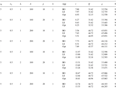
3. Numerical illustrations
A testbed of eight problems and the results obtained are presented in Table 1. For each of these it was assumed that demand in a review interval (and hence in lead time) was normally distributed. It was also assumed that demand X during the period of risk (the lead time demand plus the under-shoot) was normally distributed, with mean and variance given, from Eqs. (1)}(6), by
k"¸k
noting that, for a normal distribution,E(X3 I)"k3I #3k
Ip2I. Numerical work on other problems re-inforce the general"ndings discussed below.
For each problem we evaluated the policy arising from three di!erent approaches (App)}BO repres-ents an initial solution based on r"r
BO and Q"EOQ, LS represents an initial solution based onr"r
Table 1
Some illustrative numerical results (see text for details) k
I pI ¸ A p h App r Q g SL
5 0.5 1 100 10 1 BO 7.00 31.62 32.554 97.16
LS 7.97 31.62 32.755 98.67
Opt 6.93 32.15 32.550 97.08
5 0.5 1 100 20 1 BO 8.27 31.62 33.394 99.00
LS 8.63 31.62 33.443 99.30
Opt 8.23 32.32 33.386 98.97
5 0.5 1 200 10 1 BO 5.56 44.72 45.051 95.64
LS 7.63 44.72 45.486 98.74
Opt 5.51 44.95 45.051 95.56
5 0.5 1 200 20 1 BO 7.73 44.72 46.116 98.84
LS 8.31 44.72 46.212 99.31
Opt 7.69 45.37 46.111 98.81
5 0.5 2 100 10 1 BO 11.97 31.62 32.598 97.02
LS 13.00 31.62 32.809 98.60
Opt 11.90 32.18 32.593 96.93
5 0.5 2 100 20 1 BO 13.31 31.62 33.480 98.95
LS 13.69 31.62 33.531 99.27
Opt 13.26 32.36 33.471 98.92
5 0.5 2 200 10 1 BO 10.47 44.72 45.066 95.43
LS 12.64 44.72 45.522 98.67
Opt 10.41 44.96 45.065 95.34
5 0.5 2 200 20 1 BO 12.74 44.72 46.183 98.78
LS 13.35 44.72 46.285 99.28
Opt 12.70 45.41 46.178 98.75
optimal solution (subject to the assumptions and approximations in the model) obtained by our pol-icy-iteration algorithm from an initial solution
} this typically required "ve iterations to obtain results for which the order quantity is correct to"ve places of decimal. The last column (SL) gives the resulting stock service level (the percentage of demand met).
All the above policies incorporated the asymp-totic approximation for the undershoot. One point to note is that BO gives solutions which are very close to the ones given by Opt and consistently better than those given by LS. Policies which did not make an adjustment for the undershoot pro-duced costs which were some 2}3% higher than
those for equivalent policies adjusted for under-shoot}not surprisingly suggesting lower re-order levels than were required. Policies which employed an iterative scheme along the lines discussed in [4, pp. 168}172], with the adjustment for undershoot, generally produced results which were poorer than BO but slightly better than LS. A solution method based on optimising r (iteratively), subject to Q"EOQ and retaining ELS(r) in the denominator of (22), produced no measurable improvement on BO.
Firstly, decreasing the review interval required us to contravene assumption (ii) of Section 2.2, since the probability of negative demand increases mark-edly as the time interval tends to zero. Secondly (but related to the "rst point), the asymptotic ex-pression for the mean undershoot does not tend to zero, as the time interval tends to zero, but tends to
p2/2k, wherekandp2are the mean and variance of demand per unit time. We do not here o!er a for-mulation for a continuous review normal/Wiener demand model but just draw attention to the need for care in setting out the assumptions and analysis required for such a model to be logically consistent.
We used readily available routines for calculat-ing and invertcalculat-ing ELS(r) and PSO(r) for the normal distribution (see, for example, [10] pp. 69}71). Al-though we have concentrated on the normal distri-bution equivalent routines are available for other distributions, such as the gamma family of distribu-tions.
4. Conclusions
We have considered a periodic-review, continu-ous-demand, lost-sales model with a"xed lead time and at most one order outstanding and derived a formulation which is structurally the same as that for the equivalent continuous-review model. We have proposed a novel solution methodology, based on policy iteration. In numerical work we have established that a solution based on the eco-nomic order quantity and a simple calculation for the re-order level (our BO approach) gives solu-tions which are very close to optimal under a wide range of parameter settings and which should
suf-"ce for most practical purposes. One key area
which requires further investigation is how the analysis for this model might be extended to allow for the possibility of more than one replenishment order being outstanding at any time.
References
[1] F. Janssen, R. Heuts, T. de Kok, On the (R,s,Q) inventory model when demand is modelled as a compound Bernoulli process, European Journal of Operational Research 104 (1998) 423}436.
[2] T.E. Morton, The near-myopic nature of the lagged-pro-portional-cost inventory problem with lost sales, Opera-tions Research 19 (1971) 1708}1716.
[3] S. Nahmias, Simple approximations for a variety of dynamic lead time lost-sales inventory models, Operations Research 27 (1979) 904}924.
[4] G. Hadley, T.M. Whitin, Analysis of Inventory Systems, Prentice-Hall, Englewood Cli!s, NJ, 1963.
[5] E.A. Silver, R. Peterson, Decision Systems for Inventory Management and Production Planning, 2nd Edition, Wiley, New York, 1985.
[6] R.J. Tersine, Principles of Inventory and Materials Man-agement, 4th Edition, Prentice-Hall, Englewood Cli!s, NJ, 1994.
[7] S. Nahmias, Production and Operations Analysis, 3rd Edition, Irwin, Chicago, 1997.
[8] D. Beyer, An inventory model with Weiner demand pro-cess and positive lead time, Optimization 29 (1994) 181}193.
[9] K. Rosling, The (r,Q) inventory model with lost sales, Lund Institute of Technology, P.O. Box 118, S-221 00 Lund, Sweden, 1997.
[10] H.C. Tijms, Stochastic Models, Wiley, Chichester, 1994. [11] S.M. Ross, Applied Probability Models with Optimality
Applications, Holden-Day, San Francisco, CA, 1970. [12] I. Sahin, Regenerative Inventory Systems: Operating
Characteristics and Optimization, Springer, New York, 1990.