Full Terms & Conditions of access and use can be found at
http://www.tandfonline.com/action/journalInformation?journalCode=ubes20
Download by: [Universitas Maritim Raja Ali Haji] Date: 12 January 2016, At: 23:32
Journal of Business & Economic Statistics
ISSN: 0735-0015 (Print) 1537-2707 (Online) Journal homepage: http://www.tandfonline.com/loi/ubes20
Distributional Dominance With Trimmed Data
Frank A Cowell & Maria-Pia Victoria-Feser
To cite this article: Frank A Cowell & Maria-Pia Victoria-Feser (2006) Distributional Dominance With Trimmed Data, Journal of Business & Economic Statistics, 24:3, 291-300, DOI:
10.1198/073500105000000207
To link to this article: http://dx.doi.org/10.1198/073500105000000207
Published online: 01 Jan 2012.
Submit your article to this journal
Article views: 39
View related articles
Distributional Dominance With Trimmed Data
Frank A. C
OWELLLondon School of Economics and Political Science, Houghton Street, London WC2A 2AE, U.K. (f.cowell@lse.ac.uk)
Maria-Pia V
ICTORIA-F
ESERHEC, University of Geneva, 40 Bd du Pont d’Arve, CH-1211, Geneva, Switzerland (maria-pia.victoriafeser@hec.unige.ch)
Distributional dominance criteria are commonly applied to draw welfare inferences about comparisons, but conclusions drawn from empirical implementations of dominance criteria may be influenced by data contamination. We examine a nonparametric approach to refining Lorenz-type comparisons and apply the technique to two important examples from the Luxembourg Income Study database.
KEY WORDS: Distributional dominance; Lorenz curve; Robustness.
1. INTRODUCTION
This article addresses the issue of how practical comparisons of income distributions can be founded on a sound statistical and economic base when there is good reason to believe that the data in at least one of the distributions are “dirty.” Dirt includes the possibility of obvious gross errors in the data (such as arise from coding or transcribing mistakes) and also other more in-nocuous observations that in some sense do not really belong to the income dataset. The problem is often handled prag-matically; some empirical studies have concentrated on a sub-set of the distribution delimited either by population subgroup (e.g., taking-prime-age males only) or by arbitrarily excluding some of the data in the tails (Gottschalk and Smeeding 2000). Although this research technique seems sensible, the question of whether it is appropriate remains open—“appropriateness” here being understood in terms of the statistical properties of the underlying economic criteria. This question matters because the economic criteria are used explicitly or implicitly to make normative judgments and perhaps policy recommendations.
Cowell and Victoria-Feser (2002) set the conditions under which welfare judgments are valid with model contamination (which includes the dirty data case) and concluded that second-order rankings, such as Lorenz curves, are highly sensitive to data contamination in the tail of the distributions. Starting from this result, we propose a formalization of the practical but ad hoc procedure of trimming with a family of ranking statistics.
In this article we develop the relationship between economic ranking principles and statistical tools to derive a practical method for making distributional comparisons in the presence of data contamination. This method uses a family of dominance comparisons based on the statistical concept of the trimmed mean. The basic methodology is set out in Section 2. Consid-erations of data contamination and their likely impact on the estimates of statistics associated with distributional dominance are discussed in Section 3. The application of these methods is demonstrated in Section 4 using second-order dominance and related Lorenz comparisons over time and between countries.
2. DISTRIBUTIONAL DOMINANCE WITH “DIRTY DATA”
2.1 Informal Methods
Empirical studies of income distribution use informal rank-ing criteria as a matter of routine. There are various good
rea-sons for doing so. They usually involve easy computations, and they have a direct intuitive appeal; more important, they are usually connected to deeper points that are particularly relevant to applied welfare economists. Some prominent examples of the informal approach are as follows:
• Pragmatic indices involvingquantiles. These include the semidecile ratio (Wiles 1974; Wiles and Markowski 1971) and the comparative function of Esberger and Malmquist (1972). An extreme example of the same type is therange, literally the maximum income minus the minimum in-come, but sometimes implemented in practice as a differ-ence between extreme quantiles.
• The “parade of incomes” introduced by Pen (1971). This provides a persuasive picture of snapshot inequality and of the implications of an income distribution that is changing through time (see, e.g., Jenkins and Cowell 1994). • The use ofdistributive shares(sometimes known as
quan-tile shares).
The quantile method can be explicitly linked to formal wel-fare criteria. For example, in Rawls’ work on a theory of justice there is a discussion of how to implement his famous “differ-ence principle,” which focuses on the least advantaged. To do this, Rawls himself suggested that it might be interpreted rela-tive to the median of the distribution (see Rawls 1972, p. 98). So too can the distributive shares approach; changes in the rel-ative income shares of, say, the richest and the poorest 10% slices of the distribution can be directly interpreted in terms of the principle of transfers (Dalton 1920).
2.2 A Formal Framework
Assume that the concepts of income and income receiver have been well defined. An individual’s income is a number x∈X, where X⊆R andR is the real line. LetF be the set of probability distributions (distribution functions) with sup-portX. Anincome distributionis one particular memberF∈F.
© 2006 American Statistical Association Journal of Business & Economic Statistics July 2006, Vol. 24, No. 3 DOI 10.1198/073500105000000207
291
In this approach astatisticof any distributionF∈Fis a func-tionalT(F); for example, the meanµ:F→Rgiven by
µ(F):=
x dF(x). (1)
The properties of any functionalTmay play a role in both eco-nomic and statistical interpretations. Of particular interest here is the case where the range of T is a profile of values rather than a single number as in the example of (1);Tis then afamily of statistics. Individual family members may be of interest in their own right; the behavior of the whole family when applied to a pair of distributionsFandGwill provide important infor-mation about distributional comparisons that is richer than that provided by a single real-valued functional.
The basic distributional concept used here is aranking, which amounts to a partial ordering on the space of distributions F. We use the symbolTto denote the ranking induced onFby a
statisticT, from which a number of the concepts of strict domi-nance, equivalence, and noncomparability are derived (see, e.g., Cowell and Victoria-Feser 2002). For example, T can be the quantile function
Q(F;q)=inf{x|F(x)≥q} =xq (2)
with 0≤q≤1, which defines order dominance. The first-order dominance criterion Q is sometimes considered less
than ideal, and so it is of interest to consider the second-order criterion (Cowell 2000). This is based on thecumulative income functional,
against q describes thegeneralized Lorenz curve (GLC). The relative Lorenz curve(Lorenz 1905) is obtained by standardiz-ingC(F,q)by the mean, that is,
L(F;q):=C(F;q)
µ(F) , (4)
and theabsolute Lorenz curve(Moyes 1987) by
A(F;q):=C(F;q)−qµ(F). (5)
and Stuart 1977). The (relative) Lorenz curve encapsulates the intuitive principle of the distributional-shares ranking referred to in Section 2.1. We examine the implementation of (3), (4), and (5) in Section 4.
2.3 The Approach
To assume that data will automatically give a reasonable pic-ture of the “true” picpic-ture of a distributional comparison would obviously be reckless in the extreme. A prudent applied re-searcher will anticipate that, because of miscoding and misre-porting and other types of mistakes, some of the observations will be incorrect, and this may have a serious impact on dis-tributional comparisons (Van Praag, Hagenaars, and Van Eck
1983). Obviously, if one had reason to suspect that this sort of error were extensive in the datasets under consideration, then the problem of distributional comparison might have to be abandoned because of unreliability. But it is possible that there might be a serious problem of comparison even if the amount of contamination were small, so that the data might be considered “reasonably clean.”
Let us briefly review a standard model of this type of prob-lem. This approach is based on the work of Hampel (1968, 1974), Hampel, Ronchetti, Rousseeuw, and Stahel (1986), and Huber (1981). Suppose that the “true” distributions that we wish to compare are denoted byF andG, but because of the problem of data-contamination we cannot assume that the data we have at hand have really been generated byFandG. What we actually observe instead ofFis a distribution in some neigh-borhood of F. An elementary case is one in which a mixture distribution has been constructed by combining the “true” dis-tributionFwith a point mass at incomez
Fǫ(z)= [1−ǫ]F+ǫH(z), (6)
The degenerate distribution H(z) represents a simple form of data contaminationat point z; ǫ indicates the importance of the contamination; the convex combinationF(ǫz)is the observed distribution, andFremains unobservable.
As we have noted, ifǫis large, then we cannot expect to get sensible estimates of income distribution statistics. But what if the contamination were very small? To address this question for any given statistic T, we use theinfluence function (IF), given by Then, under the given model of data contamination (6), the sta-tisticTisrobustif the IF in (8) is bounded for allz∈X.
A more reasonable formalization is whenH(z)is generalized to any distributionH. In this case, all types of model deviations and measurement errors can be considered as being included in the mixture distribution. However, the formal study of the effect of such model deviations on the statisticT would then become impossible unless some structure were given toH. Moreover, Hampel et al. (1986) showed that
sup
which means that the reduction ofH toH(z) does not reduce the information on the bias of the statisticT under model devi-ation, such as measurement errors. In other words, the IF gives information on the behavior ofTfor any “contamination” dis-tributionH.
Cowell and Victoria-Feser (1996, 2002) showed that most inequality measures are nonrobust, but most poverty indices with exogenous poverty lines are robust (see also Monti 1991). However, the nonrobustness problem is more pervasive than that which emerges in connection with inequality measures; the same type of approach can be used to show that although first-order dominance criteria are usually robust (for further
Cowell and Victoria-Feser: Distributional Dominance With Trimmed Data 293
discussion of the statistical implementation of first-order cri-teria, see Ben Horim 1990; Stein, Pfaffenberger, and French 1987), second- and higher-order dominance criteria (and asso-ciated ranking tools) are not (Cowell and Victoria-Feser 2002). Moreover, Cowell and Victoria-Feser (2002) showed that the worst bias on the second-order ranking statistics (as provided by the IF) occurs when the contamination is in the tails of the distribution. A case can then be made for adopting an approach based on trimmed distributions. This approach certainly will not prevent biases for any type of model deviation or measurement error, but will guarantee that the largest potential biases are kept under control.
3. ROBUST DISTRIBUTIONAL DOMINANCE
3.1 Trimmed Ranking Criteria
Because ranking criteria can be misleading in the presence of data contamination, it is desirable to have a procedure that en-ables one to control systematically for suspect values that may distort distributional comparisons using second-order ranking criteria. A natural approach would be to use an established tool in the statistical literature, the “trimmed mean,” and extend the idea to Lorenz curve analysis. The trimmed mean of distribu-tionFwith trimming parameterαis
¯ timator of location has intuitive appeal; one removes the αn smallest and theαnlargest observations in a sample of sizen and calculates the mean of the remaining observations. Note that limα→.5 X¯α(F)=Q(F, .5); in the limiting case, asα ap-proaches 50%, the trimmed estimate of the mean apap-proaches the median.
Likewise, considertrimmed Lorenz curvesas estimators of Lorenz curves. One must interpret the quantile and income-cumulation functions (2) and (3).α-trimming the data means thatQ(F;q)∈(Q(F;α),Q(F;1−α))and thusq∈(α,1−α). However, it makes sense to consider a more general trimming method that includes in particular the single-tailed trimming case. Indeed, this case is appropriate when one can form an a priori judgment about the nature of the contamination, for ex-ample, when contamination is assumed to affect only the lower tail of the distribution. Letαand 1− ¯α be the lower and up-per trimming, and letα:=α+(1− ¯α) be the total trimmed amount. Then theα-trimmed generalized Lorenz, Lorenz, and absolute Lorenz curves (see the similar concept of restricted dominance, discussed in Atkinson and Bourguignon 1989) for q∈(α,1− ¯α)are given by
The IF’s of these trimmed Lorenz curves will be bounded for all qbecause extreme values in the data are automatically removed for allα,1− ¯α >0. Trimmed Lorenz curves can be thought of as Lorenz curves on a restricted sample in which 100α% of the bottom observations and 100(1− ¯α)% of the top observations have been trimmed away. This practice is some-times adopted in pragmatic discussions of inequality trends. (See also the discussion of related issues by Howes 1996.) Estimates can be obtained by replacing F with the empirical distributionF(n)(x)=1n in=1H(xi)(x).
3.2 Confidence Intervals
When comparing distributions using ranking criteria, it is also important to be able to provide confidence intervals for the latter. Cowell and Victoria-Feser (2003) give formulas for sev-eral statistics, including ranking criteria for full and trimmed samples. In particular, we have that the asymptotic covariance of √nCα(F(n);q)and√nCα(F(n);q′)withq≤q′is given by curve ordinates, the asymptotic variance is
υqq′= 1
(1−α)2µ4 α
× [µ2αωqq′+cα,qcα,q′ωα¯α¯−µαcα,qωq′α¯−µαcα,q′ωqα¯], withµα =Cα(F;1− ¯α). These covariances can be estimated by their empirical counterpart (see Sec. A.1).
3.3 Choosing the Trimming Proportions
The sampling properties of the key distributional statistics can provide a simple choice criterion. Let F˜α be the trimmed distribution given by
and letT be a statistic of interest. We consider the ratio of the mean squared errors,
κ(α):= (T(F)−T(F))
2+varT(F)
(T(F)−T(F˜α))2+varT(F˜α)
. (13)
Indeed, there is no guarantee thatT(F˜α)is a consistent estima-tor ofT(F), so that not only the variances, but also the poten-tial bias of the statistics should be taken into account. (We are gratefulul to two anonymous referees for pointing this out.) The implied trade-off of robustness against efficiency enables the researcher to make an informed choice about the extent of trimming that may be reasonable in making distributional com-parisons.
Now (13) clearly implies that this choice is conditional on the specification of T. Which statistic would be appropriate? It seems reasonable to require that this be one of second-order distributional dominance, but this raises a further difficulty: There is an uncountable infinity of statisticsC(·;q), and select-ing one or a few of these appears to be arbitrary. However, there is a simple argument suggesting that one particular case is es-pecially important. Not all values ofqin the unit interval will be relevant in computing efficiency under trimming; the very process of trimming “nibbles away” some of the interval. If one is interested in trimming of arbitrary size, then it seems to be of particular interest to examine cases whereT(F˜α)is well de-fined for arbitraryα. In the case of a balanced trim, this implies focusing attention onC(·;.5)or its relative Lorenz counterpart C(·;.5)/µ(·).
κ(α)also depends on the underlying income distributionF. For the purposes of illustrating the technique and to obtain an idea of the efficiency losses involved, we used a number of ex-amples of the Dagum type I distribution given by
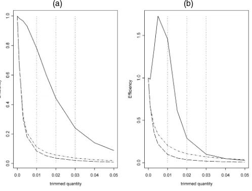
f(x;β, λ, δ)=βδλ−βxβδ−1(1+λ−1xδ)−(β+1). (14) We have (see Kleiber and Kotz 2003)Q(F;q)=λ1/δ(q−1/β− 1)−1/δandC(F;1)=λ1/δŴ(β+1/δ)Ŵ(1−1/δ)/ Ŵ(β), which were used to compute the theoretical values ofT(F). Two ex-amples are illustrated in Figure 1. From these two simulated datasets, we computed the sampling variances for the trimmed and untrimmed cases, with lower, upper, and balanced trims.
The results are illustrated in Figure 2, where the vertical axis gives estimated values ofκ(α)as defined in (13). One can see
(a) (b)
that the estimated efficiency loss (or gain) depends on the un-derlying model and the type of trim. For small trimming quanti-ties, it is not very large; for larger trimming quantiquanti-ties, it can be either quite large or reasonable. The efficiency loss is smaller with lower trimming, which for more symmetric distributions [like the Dagum(8,4,8)] can even be greater than 1! It is dif-ficult to draw a general conclusion, however, and the results presented here can provide at most a rough guideline.
4. EMPIRICAL APPLICATION
The trimming approach offers a practical tool for comparing income distribution when one wants an explicit control for tak-ing into account the influence of outliers. We use the analysis of Section 3 to more carefully examine two aspects of conven-tional wisdom concerning comparisons of income distribution. In both cases the data are taken from the Luxembourg Income Study (LIS) database and refer to real income per equivalent adult distributed among individuals (see Sec. A.2).
4.1 Cross-Country Comparison: Sweden and Germany
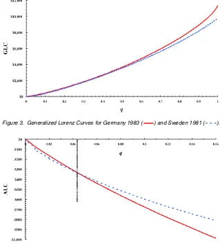
The received wisdom suggests that 1980s Sweden was more equal than Germany. But is this actually borne out by the data, and if so, what are the implications for standard wel-fare comparisons? To investigate this, we use data for Swe-den 1981 and (West) Germany 1983. As shown in Figure 3, we have FGERMANY CFSWEDEN; the German income
distri-bution second-order (generalized Lorenz) dominates that for Sweden. This conclusion is robust under trimming. But the picture is different if we attempt to apply the criterion of ab-solute Lorenz dominance. From the untrimmed data, we find FSWEDEN⊥AFGERMANY but under a very slight trimming of
both tails, it is clear that Sweden absolute Lorenz dominates Germany FSWEDENA.005 FGERMANY (compare Figs. 4 and 5).
Currency units are 1981 U.S. dollars.
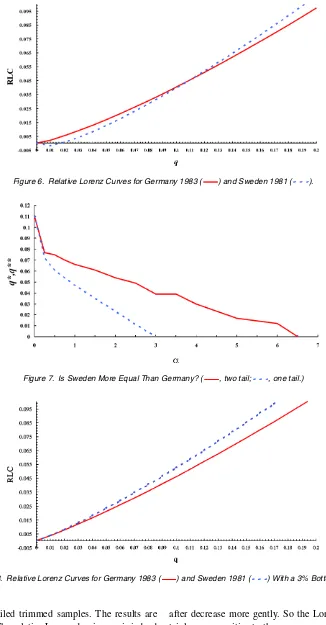
What of inequality? As Figure 6 shows, there is an ambiguity for the raw dataFSWEDEN⊥LFGERMANY, which is due to a
sin-gle intersection of the relative Lorenz curves. Figure 7 depicts
Cowell and Victoria-Feser: Distributional Dominance With Trimmed Data 295
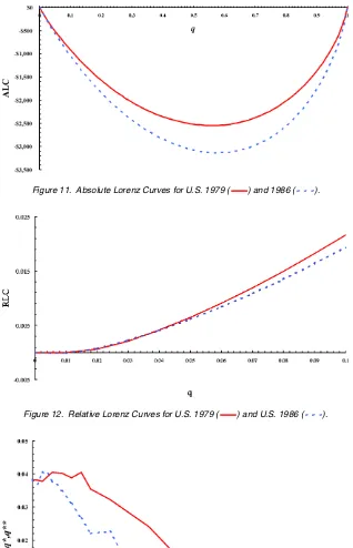
Figure 3. Generalized Lorenz Curves for Germany 1983 ( ) and Sweden 1981 ( ).
Figure 4. Absolute Lorenz Curves for Germany 1983 ( ) and Sweden 1981 ( ).
Figure 5. Absolute Lorenz Curves With .5% Balanced Trimming for Germany 1983 ( ) and Sweden 1981 ( ).
thetruncation profiles, the position of the switchpoint (where the relative Lorenz curves intersect) for two types of trim, ex-pressed as functions ofα−q∗∗(·)for the balanced two-tailed trim (solid curve) andq∗(·)for the one-sided lower-tailed trim (dotted curve). Denote the points where the truncation profiles intersect the horizontal axis byα∗∗andα∗. Then
q∗∗(0)=q∗(0)=.11,
q∗(α)=0, α≥α∗=.030,
and
q∗∗(α)=0, α≥α∗∗=.065.
We haveFSWEDENLα FGERMANY only if a trimming of 3% of
the observations is carried out on the lower tail (see Fig. 8), or a balanced trimming of 6.5%. May we say that Sweden is less unequal than Germany? Consider two points here.
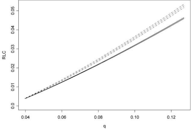
First, we apply the analysis of Section 3.2 to compute con-fidence intervals for the RLC of Germany 1983 and Sweden
Figure 6. Relative Lorenz Curves for Germany 1983 ( ) and Sweden 1981 ( ).
Figure 7. Is Sweden More Equal Than Germany? ( , two tail; , one tail.)
Figure 8. Relative Lorenz Curves for Germany 1983 ( ) and Sweden 1981 ( ) With a 3% Bottom Trim.
1981 on 3% bottom-tailed trimmed samples. The results are presented in Figure 9. The relative Lorenz dominance is indeed significant, except for the first q. This result is not surprising, because usually the sample sizes are large and thus the stan-dard errors are small. If dominance is not significant, then this should appear at the smallest or the largestqvalues.
Second, note the behavior of the truncation profiles. Both q∗∗andq∗initially fall rapidly forαvery close to 0 and
there-after decrease more gently. So the Lorenz comparison is cer-tainly very sensitive to the presence or absence of the first few observations (in either the one- or two-tailed case), but the is-sue is clearly not just one of hypersensitivity to very small in-comes. It seems unreasonable to suppose that the true picture is of strict Lorenz dominance, in that at least 1,000 observations would have to be discarded from the German data (n≃42,000) for this conclusion to obtain.
Cowell and Victoria-Feser: Distributional Dominance With Trimmed Data 297
Figure 9. RLC of Germany 1983 ( ) versus Sweden 1981 ( ) With Confidence Intervals.
4.2 Inequality Over Time: The U.S. in the 1980s
Of course, the same technique may be applied to compar-isons within one country but between two points in time. In the United States, the conventional wisdom is perhaps even sharper in its sketch of recent events; inequality rose over the 1980s (DeNavas-Walt and Cleveland 2002; Weinberg 1996). Again, the fact is—perhaps surprisingly—that the raw data do not reveal an unambiguous increase in inequality in the stan-dard sense of relative Lorenz dominance. It may appear that this is due principally to the presence of negative incomes in the first centile group. As we will see, this is not quite the whole story. Note first thatFUS86⊥CFUS79; we do not have first- or second-order distributional dominance (see Fig. 10; the gener-alized Lorenz curves intersect at aboutq=.02, .85, etc.), but FUS79AFUS86(see Fig. 11). Again, monetary units are 1981 U.S. dollars. In addition, Figure 12 shows thatFUS86⊥LFUS79. The trimming procedure is more complex. The issue of neg-ative incomes is disposed of by a very modest (<.5%) trim, but there remains an issue of multiple intersections of the rela-tive Lorenz curves at the bottom tail (with intersections between
q=.01 andq=.02 andq=.03 andq=.04). Figure 13 plots q∗∗(α)andq∗(α)in this case. In view of the multiple intersec-tions, these values are interpreted as the maximum switchpoint between the two Lorenz curves for each value ofα. We find that
α∗∗=.06 andα∗=.03. The outcome of theα-trimming pro-cedure is interesting in that—in contrast to the Germany ver-sus Sweden example—neither q∗∗(·)nor q∗(·)is monotonic. After dropping some 300–350 observations (3%) in the single-tailed trimming, or 600–700 observations (6%) in the two-single-tailed trimming, one may then conclude that FUS79Lα FUS86 (see Fig. 14). However, so much would have to be trimmed in either case that again it appears unreasonable to suppose that the true picture is one of strict Lorenz dominance.
There are some interesting points in common with the Germany-versus-Sweden example. First, for values ofαin the range [0, .01], we find a relationship between the switchpoint and α, which is clearly different from the relationship that holds in the neighborhood of the points α∗∗ andα∗. Second, the shape of the two-tailed trimming truncation profile closely follows that of the one-tailed trimming. On multiplying by 12
Figure 10. U.S. 1986 ( ) Does Not Second-Order Dominate U.S. 1979 ( ).
Figure 11. Absolute Lorenz Curves for U.S. 1979 ( ) and 1986 ( ).
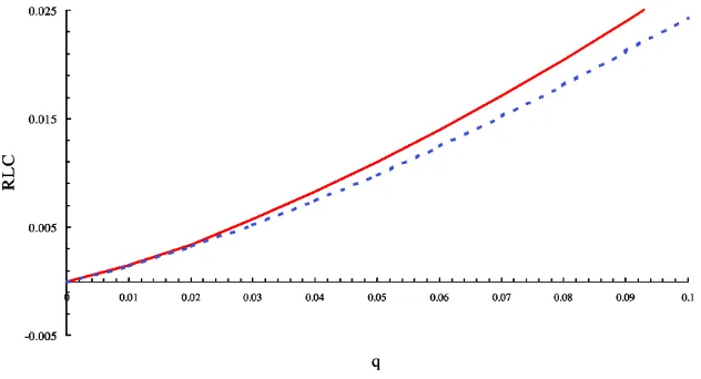
Figure 12. Relative Lorenz Curves for U.S. 1979 ( ) and U.S. 1986 ( ).
Figure 13. Did Inequality Rise in the U.S.? ( , two tail; , one tail.)
the horizontal scale of the graph of q∗∗(·), we find that it lies extremely close to that ofq∗(·); dropping 2α% of the sample in a two-tailed trimming has almost exactly the same impact on the Lorenz intersection as droppingα% of the sample in a lower-tailed trimming. Third, all of the action appears to come from the lower tail. In the distributional comparisons reported in Sections 4.1 and 4.2 we also carried out an upper-tailed ex-periment; here the hypothesis is that the data contamination is
concentrated in the high incomes and can be interpreted as po-tentially misreported data. However, in this case the ranking results turned out to be insensitive to the trim.
5. CONCLUSION
Given that second-order distributional-dominance criteria are known to be nonrobust, it is important to have practical
Cowell and Victoria-Feser: Distributional Dominance With Trimmed Data 299
Figure 14. Relative Lorenz Curves for U.S. 1979 ( ) and U.S. 1986 ( ) With a 2% Bottom-Tailed Trimming.
ods of coping with the impact of potentially “dirty” data in ei-ther tail of an income distribution. One-tailed or two-tailed (i.e., balanced) trimming provides an obvious way to extend the sim-ple distributional-dominance criteria. In effect, the researcher has the option of trading off efficiency of the distributional-dominance statistic with robustness. In this way one can place intuition about comparisons of empirical Lorenz curves on an appropriate analytical foundation. Another approach would in-volve trying to parameterize the upper or lower tail of the income distribution using robust estimation. We treated this ap-proach in an earlier article (Cowell and Victoria-Feser 2001).
ACKNOWLEDGMENTS
This work was partially supported by ESRC grant R000 23 5725. The second author is supported in part by Swiss National Fund grants 610-057883.99 and PP001-106465. The authors thank the staff of the Luxembourg Income Study and Jean-Marc Falter for cooperation with the data analysis, as well as Julie Litchfield and Ceema Namazie for research assistance.
APPENDIX
A.1 Computational Method
When using a database such as the LIS database, from which the microdata cannot be recovered directly, LC or RLC with confidence intervals at each chosenqcan be computed follow-ing this procedure:
1. Define the percentilesp (say p=0, .01, .02, . . . ,1) and trimming proportionsαand 1− ¯α.
2. Extract the personal incomes and weights from the data-base and sort the incomes and weights by incomes. 3. Define a new variable,empperc, composed of the
cumu-lative weights, and divide all elements by the maximum, that is, the last element. Keep only the incomes and the weights for whichemppercis betweenαandα¯. This de-fines the trimmed incomes,trinc, and weights,trwgt. 4. Define tottrwgt as the sum of all trwgt and define
nbtrincas the number of elements intrinc.
5. Define a new variable,trempperc, composed of the cu-mulativetrwgt, and divide all elements by the maximum, that is, the last element (and keep the value of the maxi-mum of the cumulativetrwgtin saytotweight).
6. For each percentilep>0, then do the following:
a. Select the elements of trincand trwgt for which tremppercis between p and the previous p; for exam-ple, forp=.56,tremppercis between.56 and 0.55. Call thesetrincpandtrwgtp.
b. Define m1p as the sum of trincp·trwgtp divided
bytottrwgt,m2pas the sum oftrincp·trincp·trwgtp
di-vided bytottrwgt, andxpas the maximum oftrincp.
7. Defineq=α+(1−α)p. Then forq> α, estimatecα,qby
the cumulative sum of them1p,p≤ (q1−−αα) andcα,α=0, and estimate sα,q by the cumulative sum of the m2p,
p≤(q1−α
−α)andsα,α=0. Note thatµα=cα¯.
The 95% confidence intervals for the GLC and the RLC are
(cq−1.96ωqq;cq+1.96ωqq)and(cq/µα−1.96υqq,cq/µα+ 1.96υqq), in whichωqq (and thusυqq) are estimated using the
estimates ofcα,qandsα,q. Note thatm1pand/orm2p can take
very large values depending on the measurement scale of the incomes. For numerical reasons, it may be useful to divide all incomes by a properly chosen quantity.
A.2 Data Specification
LIS permits comparison of different countries’ income distri-butions based on consistent international definitions of income and the income receiver. Accordingly, the same basic specifica-tions were used for both the Germany and Sweden and the U.S. 1979 and U.S. 1986 comparisons in Section 4. The sample sizes were as follows:
Germany 1983: 42,752 Sweden 1981: 9,625 U.S. 1979: 15,928 U.S. 1986: 12,600.
The income distributions were formed using the follow-ing concept of equivalized incomes (Buhmann, Rainwater,
Schmaus, and Smeeding 1988; Coulter, Cowell, and Jenkins 1992):
y= hhy hhsizeα,
wherehhyis net family (unit) income after tax,hhsize is the number of persons in the family unit, andα=.5. Each observa-tion is given a weight,indwgt=hhsize∗hweight, to obtain dis-tributions of income across individuals (Cowell 1984; Danziger and Taussig 1979). The variablehweightis the family unit sam-ple weight.
For calculating distributions for different years and in dollars, the following data from the IMF Year Book 1994 were used:
1981 1983
[Received May 2003. Revised August 2005.]
REFERENCES
Atkinson, A. B., and Bourguignon, F. (1989), “The Design of Direct Taxation and Family Benefits,”Journal of Public Economics, 41, 3–29.
Ben Horim, M. (1990), “Stochastic Dominance and Truncated Sample Data,”
Journal of Financial Research, 13, 105–116.
Buhmann, B., Rainwater, L., Schmaus, G., and Smeeding, T. (1988), “Equiv-alence Scales, Well-Being, Inequality and Poverty: Sensitivity Estimates Across Ten Countries Using the Luxembourg Income Study (LIS) Database,”
Review of Income and Wealth, 34, 115–142.
Coulter, F. A. E., Cowell, F. A., and Jenkins, S. P. (1992), “Equivalence Scale Relativities and the Extent of Inequality and Poverty,”Economic Journal, 102, 1067–1082.
Cowell, F. A. (1984), “The Structure of American Income Inequality,”Review of Income and Wealth, 30, 351–375.
(2000), “Measurement of Inequality,” inHandbook of Income Distrib-ution, eds. A. B. Atkinson and F. Bourguignon, Amsterdam: North-Holland, pp. 87–166.
Cowell, F. A., and Victoria-Feser, M.-P. (1996), “Robustness Properties of In-equality Measures,”Econometrica, 64, 77–101.
(2001), “Robust Lorenz Curves: A Semi-Parametric Approach,” Dis-tributional Analysis Discussion Paper 50, STICERD, London School of Eco-nomics.
(2002), “Welfare Rankings in the Presence of Contaminated Data,”
Econometrica, 70, 1221–1233.
(2003), “Distribution-Free Inference for Welfare Indices Under Com-plete and IncomCom-plete Information,” Journal of Economic Inequality, 1, 191–219.
Dalton, H. (1920), “Measurement of the Inequality of Incomes,”Economic Journal, 30, 348–361.
Danziger, S., and Taussig, M. K. (1979), “The Income Unit and the Anatomy of Income Distribution,”Review of Income and Wealth, 25, 365–375. DeNavas-Walt, C., and Cleveland, R. W. (2002),Money Income in the United
States: 2001, Current Population Reports: Consumer Income P60-191, Washington, DC: Census Bureau.
Esberger, S. E., and Malmquist, S. (1972),En Statisk Studie av Inkomstutvek-lingen, Stockholm: Statisk Centralbyr å n och Bostadssyrelsen.
Gottschalk, P., and Smeeding, T. M. (2000), “Empirical Evidence on Income Inequality in Industrialized Countries, inHandbook of Income Distribu-tion, eds. A. B. Atkinson and F. Bourguignon, Amsterdam: North-Holland, Chap. 3.
Hampel, F. R. (1968), “Contribution to the Theory of Robust Estimation,” un-published doctoral thesis, University of California, Berkeley, Dept. of???.
(1974), “The Influence Curve and Its Role in Robust Estimation,” Jour-nal of the American Statistical Association, 69, 383–393.
Hampel, F. R., Ronchetti, E. M., Rousseeuw, P. J., and Stahel, W. A. (1986),
Robust Statistics: The Approach Based on Influence Functions, New York: Wiley.
Howes, S. R. (1996), “The Influence of Aggregation on the Ordering of Distri-butions,”Economica, 63, 253–272.
Huber, P. J. (1981),Robust Statistics, New York: Wiley.
Jenkins, S. P., and Cowell, F. A. (1994), “Dwarfs and Giants in the 1980s: The UK Income Distribution and how It Changed,” Fiscal Studies, 15, 99–118.
Kendall, M., and Stuart, A. (1977),The Advanced Theory of Statistics, London: Griffin.
Kleiber, C., and Kotz, S. (2003),Statistical Size Distributions in Economics and Actuarial Sciences, Hoboken, NJ: Wiley.
Lorenz, M. O. (1905), “Methods for Measuring Concentration of Wealth,” Jour-nal of the American Statistical Association, 9, 209–219.
Monti, A. C. (1991), “The Study of the Gini Concentration Ratio by Means of the Influence Function,”Statistica, 51, 561–577.
Moyes, P. (1987), “A New Concept of Lorenz Domination,”Economics Letters, 23, 203–207.
Pen, J. (1971),Income Distribution, London: Allen Lane.
Rawls, J. (1972),A Theory of Justice, Oxford, U.K.: Oxford University Press. Stein, W. E., Pfaffenberger, R. C., and French, D. W. (1987), “Sampling Error
in First-Order Stochastic Dominance,”Journal of Financial Research, 10, 259–269.
Van Praag, B. M. S., Hagenaars, A. J. M., and Van Eck, W. (1983), “The Influ-ence of Classification and Observation Errors on the Measurement of Income Inequality,”Econometrica, 51, 1093–1108.
Weinberg, D. H. (1996),A Brief Look at U.S. Postwar Income Inequality, Cur-rent Population Reports: Household Economic Studies P60-191, Washing-ton, DC: Census Bureau.
Wiles, P. J. D. (1974),Income Distribution, East and West, Amsterdam: North-Holland.
Wiles, P. J. D., and Markowski, S. (1971), “Income Distribution Under Com-munism and Capitalism,”Soviet Studies, 22, 344–369, 485–511.