Quantifying a Deca
de of Land Cover
Change in Ghana’s Amanzule Region,
2002 – 2012
Y.Q. Wang,, Christopher Damon,, Glenn Archetto, Justice Nana Inkoom, Donald Robadue Jr. , Hilary Stevens, and Kofi Agbogah
This publication is available electronically on the Coastal Resources Center’s website at
http://www.crc.uri.edu
For more information on the Integrated Coastal and Fisheries Governance project, contact: Coastal Resources Center, University of Rhode Island, Narragansett Bay Campus, 220 South Ferry Road, Narragansett, Rhode Island 02882, USA. Brian Crawford, Director International Programs at [email protected]; Tel: 401-874-6224; Fax: 401-874-6920.
For additional information on partner activities:
WorldFish: http://www.worldfishcenter.org Friends of the Nation: http://www.fonghana.org Hen Mpoano: http://www.henmpoano.org Sustainametrix: http://www.sustainametrix.com
Citation: Wang*, Y.Q., Damon*, C., Archetto, G., Inkoom, J., Robadue, D., Stevens, H., and Agbogah,K. (2013) Quantifying a Decade of Land Cover Change in Ghana’s Amanzule Region, 2002-2012. USAID Integrated Coastal and Fisheries Governance Program for the Western Region of Ghana. Narragansett, RI: Coastal Resources Center, Graduate School of Oceanography, University of Rhode Island. 20 pp.
*Contacts: [email protected]; [email protected], Department of Natural Resources Science, University of Rhode Island, Kingston, RI 02881, USA
Table of Contents
Study Location ... 1
Land Cover Change Detection ... 1
Data Preparation... 1
Detecting Change ... 3
Results and Discussion ... 4
Re-Examination ... 4
Reducing Clutter ... 6
Conclusion ... 8
Resources ... 9
Appendix A: ... 10
Appendix B: ... 12
List of Figures Figure 1: Map of the Amanzule wetland complex in Ghana's Western Region. ... 1
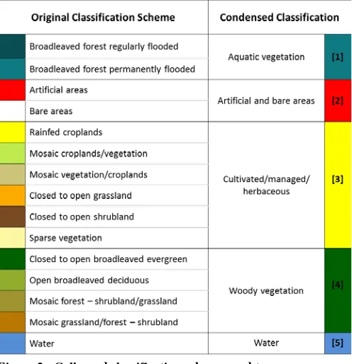
Figure 2: Collapsed classification scheme used to highlight areas of change. ... 2
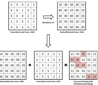
Figure 3: The change detection process using matrices to represent the input and output raster datasets. Areas of change have been highlighted in red in the final output. ... 3
Figure 4: Change matrix where all persistent classes have been set to "0" isolating locations where change has occurred. ... 3
Study Location
The Amanzule is a coastal wetland complex in Ghana’s Western Region (Figure 1) near the border with neighboring Côte d’ Ivoire. Even with its close proximity to the coast, the wetland is largely a freshwater system except along its
southeastern terminus where the outlet parallels the coast before finally emptying into the sea near Azulewanu. The ecosystem is composed of several wetland categories including peat, swamp and mangrove forests and holds Ghana’s only known peat swamp forest and the country’s largest intact swamp forest (GhanaWestCoast.com).
Despite its ecological significance, the area is not without environmental pressures. An upland diversion of the Bosoko River in 2001 led to a lowering of water levels, reduced freshwater fish catches and a change in the downstream species composition (Mckeown and Ntiri, 2005). In addition, there has been a rapid expansion in the development of the offshore oil and gas fields, and the Amanzule region has been identified as a prime terminus for pipelines extending from the Tano Deepwater and West Cape Three Points development blocks.
Land Cover Change Detection
The change detection analysis was an attempt to quantify how the land cover had changed in the Amanzule Region between 2002 and 2013. This project leveraged work from an earlier study to develop a baseline land cover map for Ghana’s Western Region as part of the Hen Mpoano Project. Hen Mpoano, or “Our Coast, Our Future” was a three year, USAID-funded endeavor lead by the University of Rhode Island’s Coastal Resources Center to develop adaptation strategies for coastal communities (Wang et al., 2012). The 2002 land cover map of the region was developed from Landsat TM data with a 30m pixel size, while the 2013 land cover mapping was developed using RapidEye multispectral imagery with a 5m pixel size.
Data Preparation
In preparation for the change analysis, it was necessary to reformat both the TM and RapidEye classifications to match in both pixel size and spatial extent in order to compute change on a pixel-by-pixel basis. This process varied for each of the source data types.
I. TM Preparation: The classified Landsat image was modified slightly from its original 28.5m pixel size to a 30m pixel size, and the extent was trimmed to match the RapidEye imagery. In order to preserve the original classification values, a
Figure 2: Collapsed classification scheme used to highlight areas of change.
“nearest neighbor” resampling method was used, thereby shifting pixels in to alignment without modifying the original classification results.
II. RapidEye Preparation: Because change detection was computed at the pixel level, it was necessary to generalize the 5m RapidEye data to a 30m pixel resolution. To accomplish this, the data were resampled using a majority filter, allowing a good representation of land cover without unduly compromising the fidelity of the original 5m data.
III. Collapsing the classification scheme: With both datasets now perfectly aligned in both extent and resolution, computing change is possible. However, the fifteen different categories of land cover type used for the classification would result in a confusing picture, displaying both distinct transformations (forest to developed) as well as the more subtle (grassland-forest to shrubland-grassland) changes.
Because inter-category variation can be heavily influenced both by image quality and sensor type, these classes of change were deemed far less important than the macro-changes occurring across the landscape. These large-scale differences have a direct impact on the goods and services a landscape can provide, and would include such modifications as forest being converted into agricultural lands or developed areas. Figure 2 displays how the original fifteen land cover categories were collapsed for each
Figure 4: Change matrix where all persistent classes have been set to "0" isolating locations where change has occurred.
Figure 3: The change detection process using matrices to represent the input and output raster datasets. Areas of change have been highlighted in red in the final output.
Detecting Change
Change detection was a straightforward comparative analysis that employed a simple
mathematical operation on each pair of pixels. Figure 3 describes this process using matrices that represent the inputs and outputs of the operation.
At the start, both the 2002 and 2012 datasets are composed of values ranging from 1 to 5, representing the five general land cover classes. To begin, one of the two data sets is
multiplied by ten to allow differentiation between the two inputs. For this work we chose to multiply the oldest land cover dataset by 10 before proceeding, and the reason for doing so will become apparent in the results.
Simply adding the two data files together results in a new matrix of values where each digit represents both the starting and ending land cover types. Upon closer examination, two different pieces of
Data,” isolates only the locations that have changed classes during the study period and separates these areas for further investigation (Figure 4).
Results and Discussion
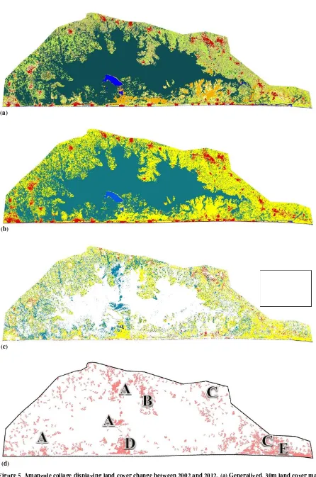
A step-wise collage showing land cover change in the Amanzule Region is displayed in Figure 5. Panels 5 a/b display the Amanzule land cover prior to the change analysis in both the original and condensed classification schemes, while panels 5 c/d exhibit the post-detection results.
Over the decade span between the 2002 and 2012 classifications, it might be expected that certain macro-scale changes would be reflected in the landscape; developed and cropland areas would tend to expand over time, and that growth would be reflected in a reduction of forested areas, grasslands, or both. In addition, it would be perfectly reasonable to
hypothesize that these changes would be greatest near the towns/villages and decrease as one moved farther afield from the population centers. However for this work, neither of these assumptions were demonstrated to be valid. Of particular note was the complete lack of spatial definition for areas where land cover change was detected — there were simply no readily identifiable patterns in either the type of change detected or the locations where change was thought to have occurred. These results (Figure 5c) indicate that change has happened universally throughout the study area, apart from the dense, regularly to permanently flooded broadleaved forest. While change surely has occurred, these initial results simply do not reflect ground conditions (May, 2013) observed during field work to collect image validation points.
Re-Examination
In an attempt to understand these results, it was necessary to revisit the Wang et al. (2012) study that developed the 2002 land cover map used as the baseline map for this work. From this, three primary factors emerged as the most likely causes for the widespread disparity between the 2002 and 2012 classifications.
(a)
(b)
(c)
(d)
classes (Kerr, 2003). Although steps were taken to mitigate these effects, difficulties remained in the ability to accurately separate adjacent land cover types in highly mosaicked environments, such as those found throughout the Amanzule (Wang et al., 2012). The second factor, was the study location itself. The Amanzule region is located in the southwestern corner of the Landsat composite used in 2012. Coincidentally, this was also the portion of the Landsat imagery that was both highly mosaicked and heavily influenced by optical
interference from haze and clouds. The final factor affecting the results was the size disparity between the two study areas -- 449,202 ha in 2012 vs. 36,507 ha for this work. By focusing on a much smaller region for this study, any classification errors from the 2012 Landsat work were distributed over a much smaller space, thus having a more noticeable impact.
While distilling the number of land cover classes used for the change detection mitigated minor spectral differences between the Landsat and RapidEye imagery, the methodology was unable to account for major classification shifts; such as from forest classes to mosaicked vegetation classes. Based on the combination of these three factors, it became apparent that it would be impossible to quantify land cover change between 2002 and 2012 with any real accuracy, even at the macro level.
Reducing Clutter
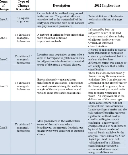
Table 1: Primary types of land cover change that were recorded between 2002 and 2012.
Description 2012 Implications
Zone A To aquatic vegetation
Occurs both at the wetland margins and in the interior. The greatest influence was observed in the western half of the study area where the haze in the Landsat imagery was most pronounced.
Better definition of freshwater wetlands and inland drainage areas.
Zone B
To cultivated / managed / herbaceous
A mixture of different forest classes that were converted to mosaic
vegetation/croplands.
Influenced by both the subjective nature of the land cover classes and the similarity of adjacent land cover types. Overall, an improved
Locations near population centers where areas of bare/sparse vegetation or mosaic forest/grassland/shrubland are converted to one of the mosaic cropland classes.
It would be reasonable to expect these transitions as population centers expand outward, but it is unclear whether these
differences reflect true change or are simply the result of a better classification.
Zone D
To cultivated / managed / herbaceous
Bare and sparsely vegetated areas transformed to grasslands. These zones are most prominent along the southern margin of the study area where inland wetland areas abut sandy coastal soils.
These locations are temporarily flooded during the rainy season with sheet flow from the interior. Depending on the time of year or the density of the grasses, these zones can easily be mistaken for bare to sparse vegetation or water. An improvement in the delineation of this cover type.
Zone E
To cultivated / managed / herbaceous
Most pronounced in the southeastern corner of the study area where
broadleaved, permanently flooded areas (mangroves) were converted to cropland classes.
Conclusion
Resources
Ghana West Coast. “Amanzule”. http://ghanawestcoast.com.
Kerr, J.T. and M. Ostrovsky, 2003. From space to species: ecological applications for remote sensing. Trends in Ecology and Evolution 18 (6).
Mckeown, J.P and E. Ntiri. 2005. “Conflict in the diversion of the Bosoko river in the Amanzule Lake”. In A. Engel and B. Korf. Negotiation and mediation techniques for natural resource management. DFID/FAO Livelihood Support Programme. Rome, FAO. Wang, Y.Q., C. Damon, G. Archetto, D. Robadue, and M. Fenn. 2012. Land cover mapping
Appendix A:
Land cover classes and descriptions used for the Amanzule land cover change detection project
Class Name Class # Class Description
Rainfed Croplands 1 Crops whose establishment and development are completely determined by rainfall.
Mosaic
Croplands/Vegetation 2
A mapping unit which contains 50-70% cropland and 20-50 percent vegetative cover
(grassland/shrubland/forest) Mosaic
Vegetation/Croplands 3
A mapping unit which contains 50-70% vegetative cover (grassland/shrubland/forest) and 20-50 cropland. Closed to Open
Broadleaved Evergreen or Semi-Deciduous Forest
4
A class representing 100-40% of the cover within a mapping unit which is comprised of broadleaved evergreen or semi-deciduous forest. The crowns can form an even or uneven canopy layer.
Open Broadleaved
Deciduous Forest 5
Between 70-60 and 40 percent of a mapping unit is covered by broadleaved deciduous forest. The crowns of the canopy are not usually interlocking. The distance between crowns can range from very small up to twice the average diameter of the crown.
Mosaic Forest –
Shrubland/Grassland 6
A mixed mapping unit which consists of 50-70% forest and 50-20% shrubland or grassland.
Mosaic
Grassland/Forest – Shrubland
7 A mixed mapping unit which consists of 50-70% grassland or forest and 20-50% shrubland. Closed to Open
Shrubland 8
Shrubland which covers 100 to 40% of a mapping unit. Shrubland is defined as woody vegetation smaller than 5 meters in height.
Closed to Open
Grassland 9
Grassland which covers 100 to 40% of a mapping unit. Grassland is defined as herbaceous cover which is 3 to .03 meters in height.
Sparse Vegetation 10 A mapping unit which contains 20-10% to 1% vegetative cover.
Broadleaved forest covering 100-40% of the mapping unit which is flooded for during a particular season with fresh or brackish water.
Closed Broadleaved Forest Permanently
12
Appendix B:
2012 Land Cover Maps