Application of Vector ...(Hartini, et al)
Application of Vector Auto Regression Model
for Rainfall-River Discharge Analysis
Sri Hartini
1, M. Pramono Hadi
2, Sudibyakto
2, Aris Poniman
11Geospasial Information Agency, Jl. Raya Jakarta – Bogor Km. 46, Cibinong, Bogor 16911
2Faculty of Geography, Universitas Gadjah Mada, Sekip Utara, Bulak Sumur, Yogyakarta
Corresponding E-mail: [email protected]
Abstract
River discharge quantity is highly depended on rainfall and initial condition of river discharge; hence, the river discharge has auto-correlation relationships. This study used Vector Auto Regression (VAR) model for analysing the relationship between rainfall and river discharge variables. VAR model was selected by considering the nature of the relationship between rainfall and river discharge as well as the types of rainfall and discharge data, which are in form of time series data. This research was conducted by using daily rainfall and river discharge data obtained from three weirs, namely Sojomerto and Juwero, in Kendal Regency and Glapan in Demak Regency, Central Java Province. Result of the causality tests shows significant relationship of both variables, those on the influence of rainfall to river discharge as well as the influence of river discharge to rainfall variables. The significance relationships of river discharge to rainfall indicate that the rainfall in this area has moved downstream. In addition, the form of VAR model could explain the variety of the relationships ranging between 6.4% - 70.1%. These analyses could be improved by using rainfall and river discharge time series data measured in shorter time interval but in longer period.
Keywords: rainfall, river discharge, VAR
Abstrak
Besar kecilnya debit sungai sangat tergantung pada hujan dan kondisi awal dari debit itu sendiri, sehingga terdapat hubungan auto-correlation. Sementara itu, proses pengalihragaman dari hujan menjadi debit aliran pada sungai membutuhkan waktu (lag)antara terjadinya hujan dan kenaikan debit sungai. Penelitian ini menggunakan modelVector Auto Regression (VAR) untuk menganalisis hubungan antara curah hujan dan debit. Model VAR dipilih dengan mempertimbangkan bentuk hubungan antara kedua variabel dan tipe data hujan maupun debit yang keduanya merupakan data deret waktu (time series). Data curah hujan dan data debit harian diperoleh dari tiga bendung yaitu Bendung Sojomerto, Bendung Juwero di Kabupaten Kendal dan Bendung Glapan di Kabupaten Demak, Provinsi Jawa Tengah. Hasil uji kausalitas menunjukkan hubungan yang signifikan baik antara pengaruh variabel curah hujan terhadap debit maupun pengaruh debit terhadap curah hujan. Hubungan kausalitas yang signifikan antara debit terhadap curah hujan mengindikasikan bahwa karakteristik hujan di wilayah ini bergeser dari hulu ke hilir. Model VAR yang terbentuk dapat menjelaskan keragaman
hubungan antara kedua variabel antara 6,4% – 70,1%. Hasil penelitian menunjukkan bahwa model statistik berpeluang
digunakan dalam peramalan hubungan hujan dan debit sungai. Analisis ini dapat dipertajam dengan menggunakan data deret waktu pada interval waktu yang lebih rapat dan periode yang lebih panjang.
Kata Kunci: hujan, debit sungai,VAR.
Introduction
The north coastal region of Central Java is an area prone to flood which is caused by heavy rainfall and tidal inundation. This research discusses about rainfall as one of the causes of flood in this area. Kodoatie & Sugiyanto (2002) states that flood can be observed based on two types of events. Flood is an event when there is inundation on a particular area that normally is not inundated, and also an
Transformation process of rainfall into a stream flow is one of interesting subjects in hydrology since it can be applied as a basis of flood forecasting. Several hydrological models have been developed either based on the process or the data availability. The first models are also known as conceptual models. Meanwhile, the second models are called as data driven model. The conceptual model has been developed for explaining the entire process of rainfall transformation into a streamflow using physical mechanism approach that represents the hydrological cycle. Among the hydrological models developed based on process are TOPKAPI (Liu & Todini, 2002) and SIMHYD, Sacramento, AWBM (Vaze et al., 2012). The data availability commonly hinders the development of conceptual model, particularly on a distributed model. The conceptual model requires comprehensive and detailed topography, hydrology and meteorology data. A statistical model has also been developed for hydrological modelling; usually by using time series data (Kar, Lohani, Goel, & Roy, 2010; Lohani, Kumar, & Singh, 2012). Statistical models generally require a set of historical observation
data to determine the system’s parameters. Statistical
models used in this system are auto-regression linier model, multiple linear regressions, moving average and Artificial Neural Network (ANN). A linier regression model is applied for developing a quantitative relationship between predictor variables and observed responses.
Related to the influence of rainfall to the stream flow as reflected by the quantity of river discharge, these two variables do not always have a linear relationship at the same time. The transformation process of rainfall into the stream flow takes some amount of time so that there is lag between the occurrence of rainfall and the increase of river discharge that measured in the river. This time lag depends on the physical and hydrological characteristics such as land cover, topography and watershed morphometric (Ko & Cheng, 2004). Beside influenced by rainfall, river discharge is also influenced by the state of river discharge conditions at the station so that there is an auto-correlation. Hence, a model is required to determine the relationship between rainfall and river discharge. The selection of a model should consider the characteristics of the data and the objectives to be obtained.
Considering the relationships between rainfall and river discharge, and the form of the rainfall and river discharge data, which are time series, the statistical model that can be applied to predict the relationship between the two variables is an auto-regression
model. Statistical models which is popularly used for the analysis of univariate time series data is Autoregressive Integrated Moving Average (ARIMA). ARIMA is a statistical model that completely ignores the independent variables in making a forecast. ARIMA applies the past and the present values of the dependent variables to produce accurate short-term forecasting. ARIMA is suitable if the observed time series data is statistically correlated each other (dependent) such as the rainfall data. ARIMA has been used in several studies of rainfall forecasting (Huda et al., 2012; Hasria, 2012).
However, a multivariate statistical model would be required in conditions where an event is influenced by more than one variable. By considering both cases, the appropriate statistical model to analyse the relationship between rainfall and river discharge is Vector Auto Regression (VAR).VAR is a statistical model that can be used to project the system variable by using time series data. VAR is also able to analyze the dynamic impacts of disturbance factors in the system variable. It can be used to understand the reciprocal relationship between variables as well as to determine the relationship between causality and impulse response of related variables and to understand the inter-relationship between variables (Hadi, 2003).
Several studies have shown the success of VAR model in proving the relationship between variables. Diani et al. (2013) and Saputro et al. (2011) used VAR models to determine the relationship between rainfalls in several stations. Adenomon (2013) and Das (2013) used VAR model to analyze relationships between rainfall and temperature. Both researches found significant relationships between rainfall and temperature. In contrast to these studies, VAR analysis in this study was used to examine the relationship between rainfall and river discharge. This model used with an assumption that the rainfall and river discharge variables are influenced by their own behaviour in the past, and that these two variables affect each other, even thought the effect is not immediate but within a certain time lag.
elevation than the weirs’ positions. Since water flows
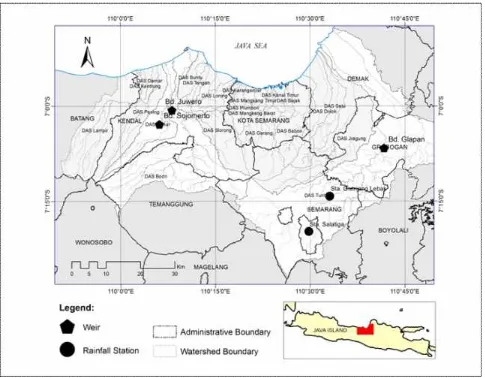
follows the slope, it is important to pay attention to the geographic positions of the weir and rainfall stations in analyzing the relationship between river discharge and rainfall. In this study, there is no rainfall station above the Juwero weir (Bodri river) so that the relationship analysis between rainfall and river discharge was only conducted based on data measured at the stations installed at the same location. A similar analysis has been conducted for Blukar watershed by using river discharge and rainfall data collected from Sojomerto weir (Blukar river), since the rainfall data collected from the upper rainfall station such as at Patean Curuk station contain many blank data. Meanwhile the analysis of the relationship between water discharge and rainfall in Tuntang watershed was done by using the river discharge data obtained from Glapan weir and rainfall data taken from Grenjeng Lebak, and Salatiga rainfall stations.
Research Method
The river discharge and rainfall data were obtained from the office of the Water Resources Centre (Pusat Sumber Daya Air/PSDA) and the Office of Meteorology and Geophysics Agency (BMKG) in Semarang, Central Java Province. Both of the discharge and rainfall data used are daily data collected in 1999-2009. However, both of these time series data were not entirely complete. Therefore, this study only used the discharge and rainfall time-series data that were in pairs as shown in Table 1. The data analysis was also performed on the combined river discharge and rainfall data to perform relationship between rainfall data collected at Grenjeng Lebak Station, Bawen Station and Salatiga Station andriver discharge data measured at the Glapan weir, Tuntang watershed. Figure 1 shows the research area and the location of the rainfall stations and weirs
.
Analysis of causality relationship between rainfall and river discharge measured at the weirs was done by using the VAR model run on Eviews version 8.
The VAR model treated all variables equally, so that there are no endogenous and exogenous variables. As an assumption in the VAR model is that the data are stationary, the initial stage in the estimation of the VAR model is examining the stationarity of the data.The next stage was determining the optimum lag in the VAR model, which was done by examining the optimum lags on each variable. Causality test was conducted to determine the causality relationship among variables. By using the stationary data, the VAR model estimations were performed using the optimum lags. The procedure of VAR analysis used refers to Startz (2013) as follows:
Unit Root Test
VAR model assume that the data is stationary, means that there is no significant change in the data. Time series data considered as stationary when the mean is relatively constant, or the data are stable during a certain period. This study applies a stationary test using the Augmented Dickey Fuller Test (ADF Test). When the data are stationary, the estimation of the VAR model uses the data at 0 (zero) order or level. However, if there is a trend on the data or the data are not stationary, the data used at the first or second differential.
Determining Optimum Lag
The optimum lag to be used in the VAR model should be determined. This research used Schwarz information criterion as an indicator in determining the length of lags. The optimum lag was determined from the lowest value of the Schwarz information criteria.
Causality Test
Causality test in the VAR model is used to determine the causality relationship between variables. Assessment of the causality relationships of the VAR model in this study carried out by using the Granger causality function.
Impulse Response Function
Impulse response function is used to determine the instantaneous influence of a variable against another, in this case are the rainfall and river discharge variables. This study used Cholesky impulse response function.
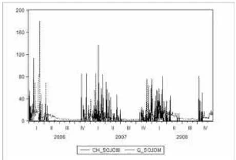
As mentioned earlier, the daily river discharge and rainfall data provided are not entirely complete. Therefore, the VAR model only used selected data that fall in pairs in a particular period which meet the requirements of the model. Both of the data used in the VAR model can be seen in Table 1, and the graph of the daily discharge and rainfall data used shown in Figure 2, Figure 3, and Figure 4.
Figure 2. Daily rainfall at Juwero station
(CH_Juwero) and daily river discharge at Juwero weir (Q_Juwero)
0 40 80 120 160 200
M2 M3 M4 M5 M6 M7 M8 M9 M10 M11 M12 M1
2005 2006
Q _G LAP AN
0 20 40 60 80 100 120 140
M2 M3 M4 M5 M6 M7 M8 M9 M10 M11 M12 M1
2005 2006
C H_S ALAT IG A
0 20 40 60 80 100 120 140
M2 M3 M4 M5 M6 M7 M8 M9 M10 M11 M12 M1
2005 2006
C H_G LE B AK
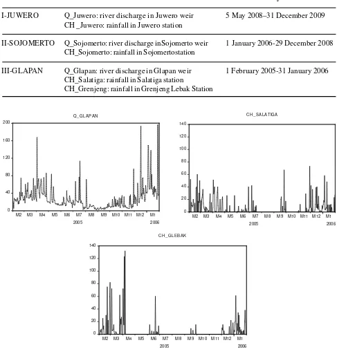
Table 1.Variables and daily data on the VAR model
VAR Model VAR Variable Daily Data
I-JUWERO Q_Juwero: river discharge in Juwero weir 5 May 2008–31 December 2009
CH _Juwero: rainfall in Juwero station
II-SOJOMERTO Q_Sojomerto: river discharge inSojomerto weir 1 January 2006-29 December 2008 CH_Sojomerto: rainfall in Sojomertostation
III-GLAPAN Q_Glapan: river discharge in Glapan weir 1 February 2005-31 January 2006 CH_Salatiga: rainfall in Salatiga station
CH_Grenjeng: rainfall in Grenjeng Lebak Station
Figure 4. Daily river discharge at Glapan weir (Q_Glapan), and daily rainfall at Salatiga station (CH_Salatiga) and Grenjeng Lebak station (CH_Glebak)
Result and Discussion
Descriptions of the result of VAR model analysis are as follow:
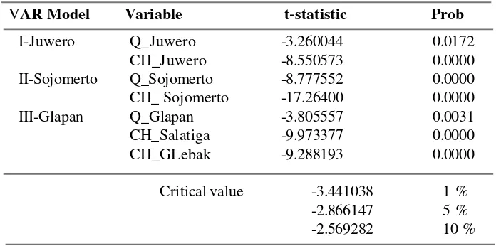
a. Unit Root Test
The ADF test was used to test the stationary variables
VAR Model Variable t-statistic Prob
I-Juwero Q_Juwero -3.260044 0.0172
CH_Juwero -8.550573 0.0000
II-Sojomerto Q_Sojomerto -8.777552 0.0000
CH_ Sojomerto -17.26400 0.0000
III-Glapan Q_Glapan -3.805557 0.0031
CH_Salatiga -9.973377 0.0000
CH_GLebak -9.288193 0.0000
Critical value -3.441038 1 %
-2.866147 5 %
-2.569282 10 %
Tabel 2. Unit Root Test at Level
b. Determination of optimum lag
The optimum lag determined by using the Schwarz information criteria and the result is shown in Table 3. The optimum lags of the VAR variables at the three watershed were 2 (Model I-Juwero), 3 (Model II-Sojomerto) and 2 (Model III-Glapan). Thus, the VAR models used those three optimum lags.
c. Granger causality test
Causality test was conducted to determine the causal relationship between the variables of the VAR model and the results shown based on its probability. The lags used in the Granger causality tests were the optimum lags. Result of the Granger causality tests is shown in Table 4.
VAR Model Schwarz Information Criteria Optimal Lag
I-Juwero 15.86510 2
II-Sojomerto 14.93847 3
III-Glapan 24.80236 2
Table 3. Optimal Lag Length
VAR Model H0 F-Stat Prob
I-Juwero 1.Q_JUWERO does not Granger Cause CH_JUWERO 4.456 0.0120 2.CH_JUWERO does not Granger Cause Q_JUWERO 48.544 3.E-20
II-Sojomerto 3.CH_SOJOM does not Granger Cause Q_SOJOM 4.422 0.0042 4.Q_SOJOM does not Granger Cause CH_SOJOM 4.978 0.0020
III-Glapan 5.CH_SALATIGA does not Granger Cause Q_GLAPAN 4.443 0.0124 6.Q_GLAPAN does not Granger Cause CH_SALATIGA 5.285 0.0055 7.CH_GLEBAK does not Granger Cause CH_SALATIGA 3.183 0.0426 8.CH_SALATIGA does not Granger Cause CH_GLEBAK 12.415 6.E-06 9.Q_GLAPAN does not Granger Cause CH_GLEBAK 3.846 0.0223 10.CH_GLEBAK does not Granger Cause Q_GLAPAN 2.559 0.0788
The results of the causality test indicates that in model I-Juwero for the relationship between CH Juwero and Q_Juwero variables, the first and second hypothesis of Ho were rejected at the probability value <5%. This shows that the Q_Juwero variable influenced to the CH_Juwero variable, and the CH_Juwero variable was influenced to the Q_Juwero variable at 95% of confidence level.
In the case of model II-Sojomerto, the relationship between Q_Sojomerto and CH_Sojomerto variables, shows that the third and fourth Ho hypothesis was rejected with the probability value <5%. It shows that the Q_Sojomerto variable influenced the CH_Sojomerto whereas the CH_Sojomerto variable also influenced the Q_Sojomerto at 95% of confidence level.
Further, the model III-Glapan model for the casualty relationship between CH_Salatiga and Q_Glapan variables, the 5th and 6thHo hypothesis were rejected at probability value of <5%. It shows that the Q_Glapan variable has influenced the CH_Salatiga and vice versa at 95% of confidence level.
The model of III-Glapan for the relationship between CH_Salatiga and CH_Glebak variables, the 7th and 8thHo hypothesis were rejected at the probability value <5%. It shows that CH_Glebak variable has influenced the CH_Salatiga variable and vice versa at 95% confidence level.
The III-Glapan model for the relationship between Q Glapan and CH_Glebak variables, the 9thHo hypothesis was rejected at the probability value of <5%, while at the 10thhypothesis Ho was rejected at the probability value of <10%. This shows that the CH_Glebak variable has influenced the Q_Glapan variable at 95% confidence level and vice versa at 90% confidence level.
a. VAR Model
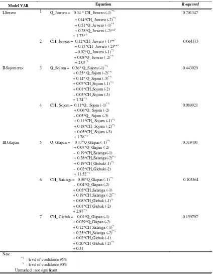
The formed of VAR models resulted from the analysis are shown in Table 5. Equation 1 shows that the CH_Juwero variable at lag 1 and 2 and the Q_Juwero variable at lag 1 and 2 show a significant influence to the Q_Juwero variable. This means that the rainfall and river discharge occurred one and two days earlier had a significant influence to the river discharge at the Juwero weir. These variables could explain the variety of water discharge in that weir by 70.13% (R-squared).
Equation 2 shows that the CH_Juwero variables at lag 1 and the Q_Juwero variable at lag 1 and 2 show significant influences to the CH_Juwero variable.
While the CH_Juwero variable at lag 2, has only a little effect to the Q_Juwero. It shows that rainfall occurred two days earlier at Juwero station and river water discharge that occurred one and two days earlier at that station had a significant influence to
today’s rainfall at that station. These variables could
explain the diversity of rainfall at the Juwero Station by 6.44% (R-squared).
Equation 3 shows that the CH_Sojom variable (at lag 1) and the Q_Sojom variable (at lag 1, 2 and 3) had significant influences to the Q_Sojom variables. Meanwhile, the CH_Sojom variable at lag 2 and 3 did not show a significant effect to the Q_Sojom variable. This shows that the river discharge at Sojomerto weir during the previous three days and the rainfall occurred one day earlier at Sojomerto
station have significant influences to the today’s river
discharge in Sojomerto weir. These variables could explain the variety of the river discharge in Sojomertoweir by 44.30% (R-squared).
Equation 4 shows that the Q_Sojom variable (at lag 1) and CH_Sojom variable (at lag 1 and 2) had significant influences to the CH_Sojom variable. Meanwhile, the Q_Sojom variable (at lag 2 and 3) and CH_Sojom variable (at lag 3)did not have the same effect to the CH_Sojom. It shows that the river discharge at Sojomerto weir at one day earlier and the rainfall occurred at one day and two days earlier at the Sojomerto station have significant influences
to the today’s rainfall in Sojomerto station. These
variables could explain the variety of rainfall in Sojomerto station by 8.99% (R-squared).
Equation 5 shows that the Q_Glapan variable (at lag 1), CH_Salatiga variable (at lag 2) and CH_Glebak variable (at lag 1) had significant influences to the Q_Glapan variable. While the Q_Glapan variable (at lag 2) and CH_Salatiga variable (at lag 1) and CH_Glebak variable (at lag 2), had insignificant effect to the Q_Glapan variable. This shows that the states of river discharge at Glapan weir and the rainfall at Grenjeng Lebak station at one day earlier, as well as the rainfall in Salatiga stations at two days earlier
had significant influences to the today’s water
discharge at Glapan weir. These variables could explain the variety of river discharge at Glapan weir by 31.94% (R-squared).
CH_Glebak variable (at lag 2), had insignificant influences to the CH_Salatiga. This shows that the rainfall occurred two days earlier at Salatiga station, and rainfall occurred one day earlier at Grenjeng Lebak station and the river discharge at Glapan weir
provide significant influence to the today’s rainfall in
Salatiga Station. These variables could explain the variety of rainfall in Salatiga Station by10.36% (R-squared).Equation 7 shows that the CH_Salatiga (at lag 1 and 2) and CH_Glebak variable (at lag 2) had
significant influences to the CH_Glebak variable. Meanwhile, the Q_Glapan variable (at lag 1 and 2) and CH_Glebak variable (at lag 1), shows insignificant influences to the CH_Salatiga. This means that the rainfall occurred at two and one day earlier at Salatiga and Grenjeng Lebak stations provide significant
influences to the today’s rainfall at Grenjeng Lebak
Station. These variables could explain the variety of rainfall variables in that station by 15.98% (R-squared).
Model VAR Equation R-squared
I-Juwero 1 Q_Juwero = 0.34 * CH_ Juwero (-1)**) + 014*CH_ Juwero (-2)**) + 0.51*Q_ Ju wero (-1)**)
+ 0.28*Q_ Ju wero (-2)**) + 1.73**)
0.701347
2 CH_ Juwero = 0.12*CH_ Juwero (-1)**) + 0.15*CH_ Juwero (-2)**)
–0.02*Q_ Juwero (-1)**) + 0.08*Q_ J uwero (-2)**)
+ 2.07*)
0.064373
II-Sojomerto 3 Q_Sojom = 0.36* Q_Sojom (-1)**) + 0.25* Q_ Sojom (-2)**)
+ 0.14* Q_ Sojom (-3)**) + 0.07*CH_Sojom (-1)**)
+ 0.01*CH_Sojom (-2) - 0.03*CH_Sojom (-3) + 1.74**)
0.443029
4 CH_ Sojom = 0.11*Q_ Sojom (-1)**) + 0.06*Q_ Sojom (-2) - 0.05*Q_ Sojom (-3) + 0.11*CH_ Sojom (-1)**)
+ 0.18*CH_ Sojom (-2)**)
+ 0.05*CH_ Sojom (-3) + 1.76**)
0.089921
III-Glapan 5 Q_Glapan = 0.47*Q_Glapan (-1)**) + 0.07*Q_ Glapan (-2) - 0.19*CH_Salatiga(-1) + 0.28*CH_Salatiga(-2)**)
+ 0.19*CH_Glebak(-1)**)
- 0.02*CH_Glebak(-2) + 11.52**)
0.319401
6 CH_ Salatiga = 0.08*Q_Glapan (-1)**) - 0.04*Q_Glapan (-2) + 0.05*CH_Salatiga (-1) + 0.19*CH_Salatiga (-2)**)
+ 0.08*CH_Glebak (-1)*)
+ 0.01*CH_Glebak (-2) + 2.87**)
0.103564
7 CH_ Glebak = 0.01*Q_Glapan (-1) + 0.029*Q_Glapan (-2) + 0.12*CH_Salatiga (-1)*) + 0.25*CH_Salatiga (-2)**) + 0.02*CH_Glebak (-1) + 0.20*CH_Glebak (-2)**) + 0.31
0.159797
Note :
**)
: level of confidence 95%
*) : level of confidence 90%
Unmarked : not significant
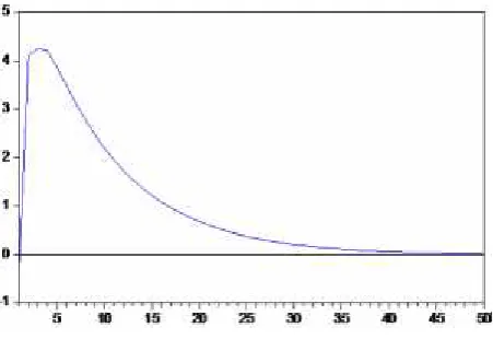
e. Impulse Response
Impulse response function was used to analyze the effect of rainfall variable to river discharge variable and vice versa. One example of the influences of rainfall to the increase of river discharge at Juwero weir can be seen in Figure 5. The increase of the rainfall significantly influenced to the increase of river discharge and it reached the peak on the second day, and then gradually decline on the rest of the days until reached its stationary at level .
used in this study statistically confirms that the increase of the river discharge is not only affected by the rainfall, but also influenced by the river discharge. This condition indicates that the increase in the discharge at the weir was also affected by the rainfall that occurs in the upstream during the previous days. This significant casualty relationship indicates that the characteristics of the rainfall in this region shifted downstream, as confirmed by the VAR model at Glapan weir. Meanwhile, the number of time lag indicates the time required from the incidence of rainfall to the measured of river discharge. As a result, the differences of the time lag of these three weirs indicated the differences of the physical and hydrological characteristics of the watersheds.
Distance factor may also affects to the measured discharge as shown in the VAR model for Glapan weir. Hadi (2006) proved the significant relationship of inter-stations correlation analysis on the rainfall and the distance. Therefore, future researches need to be developed by providing the relationship between the influenced variables and distance.
Conclusion
The VAR analysis result could determine the causality relationship between rainfall and river discharge variables. Statistically, these relationships are shown by their causality functions.The significant causality relationships between the river discharge and the rainfall variables indicated that the characteristics of the rainfall in this study area was that the rainfall occurrence moved from upstream to downstream. However, there is limitation in this study, which could affect to the result of prediction, mainly to the prediction on the peak of the river discharge reflected by the time lag. This occurred due to the data used were daily data. By using them, the rainfall is presumed to occur throughout the day, while in fact the rain could have only occurred in a few hours in each day. Similarly, the river discharge data may not be constant throughout the day. Accuracy of the prediction could increase by using data measured in shorter time interval; for example an hourly data but that collected in longer period.
Acknowledgement
The authors would like to deliver their gratitude to the Agency for Meteorology, Climatology, Geophysics (BMKG) and the Water Resource Centre (PSDA), Central Java Province, which have provided the rainfall and river discharge data used in this research. Understanding the relationship between rainfall and
river discharge is reasonably easy, since an increase of rainfall will be followed by an increase of river discharge within a certain time lag depending on physical and hydrological characteristics of watershed. The result of causality test in this study positively confirms the relationship between these variables as shown in Juwero weir. The VAR models formed could explain the variety of the river discharge variable in reasonably high percentage.The relationships between rainfall and river discharge at Sojomerto and Glapan weirs show similar behaviour, although the response was different as shown by the value of the time lag and the percentage of the variety that could be explained. The rainfall stations used to predict the discharge at Glapan weir located at the higher altitude than the weir, but the influence of the river discharge variable to the rainfall variables atSalatiga and Grenjeng Lebak stations was prominent and illustrated by both the causality relationships of the VAR models.
Statistically, the causality functions shows that the discharge variable also influence to the rainfall variable. Logically, this condition might not happen; nevertheless, the VAR model could show that the increase of the measured river discharge was also affected by its previous condition.The VAR models Figure 5. The impulse response graph of the
References
Adenomon, M. (2013). Modelling The Dynamic Relationship Between Rainfall and Temperature Time Series Data in Niger State, Nigeria. Mathematical Theory and Modeling. Vol.3 No. 4. pp. 53-70, Retrieved from http://www.iiste.org/Journals/index.php/MTM/article/view/5325, [20 August 2014].
Asdak, C. (2002). Hidrologi dan Pengelolaan Daerah Aliran Sungai. Yogyakarta: Gadjah Mada University Press.
Das D. (2013). Variation of Temperature and Rainfall in India. International Journal of Advances in Engineer-ing & Technology, Sept. 2013, Retrieved from http://www.e-ij aet.org/media/41I16-IJAET0916831_v6_iss4_1803to1812.pdf, [20 August 2014].
Diani, K. A. N., Setiawan, & Suhartono.(2013). Pemodelan VAR-NN dan GSTAR-NN untuk Peramalan Curah Hujan di Kabupaten Malang. JURNAL SAINS DAN SENI POMITS, 2 (1). Retrieved from http://ejurnal.its.ac.id/index.php/sains_seni/article/viewFile/3137/771
Hadi, Y. S. (2003). Analisis Vector Auto Regression (VAR) Terhadap Korelasi Antara Pendapatan Nasional
dan Investasi Pemerintah di Indonesia, 983/1984 – 1999/2000. Jurnal Keuangan Dan Moneter, 6 (2), 107–121. Retrieved from http://www.fiskal.depkeu.go.id/webbkf/kajian%5C7.Jonatan-2.pdf, [19 August
2014].
Hadi, M. P. (2006). Pemahaman Karakteristik Hujan Sebagai Dasar Pemilihan Model Hidrologi (Studi Kasus di
DAS Bengawan Solo Hulu). Forum Geografi, 20(1), 13–26. Retrieved from 202.154.59.182/ejournal/
files/hujan.pdf. [12/06/2010]
Hasria.(2012). Prakiraan Curah Hujan Bulanan Kota Kendari dengan Model ARIMA. Jurnal Aplikasi Fisika, 8
(1 - Februari), 25–30, Retrieved from http://jaf-unhalu.webs.com/5_JAF-_Februari_12__Hasria_.pdf,
[22August 2014].
Huda, A. M., Choiruddin, A., Budiarto, O., & Sutikno.(2012). Peramalan Data Curah Hujan dengan Seasonal Autoregressive Integrated Moving Average (SARIMA) Dengan Deteksi Outlier Sebagai Upaya Optimalisasi Produksi Pertanian di Kabupaten Mojokerto. Dalam Proceeding Seminar Nasional: Kedaulatan Pangan dan Energi. Madura: Fakultas Pertanian Universitas Trunojoyo, Retrieved from http:/ /pertanian.trunojoyo.ac.id/semnas/wp-content/uploads/PERAMALAN-DATA-CURAH-HUJAN- DENGAN-SEASONAL-AUTOREGRESSIVE-INTEGRATED-MOVING-AVERAGE-_SARIMA_-DENGAN-DETEKSI-OU.pdf, [22August 2014].
Kar, A. K., Lohani, A. K., Goel, N. K., & Roy, G. P. (2010). Development of Flood Forecasting System Using Statistical and ANN Techniques in the Downstream Catchment of Mahanadi Basin, India. Journal Water
Resource and Protection, 2010 (October), 880–887. doi:10.4236/jwarp.2010.210105
Ko, C., & Cheng, Q. (2004). GIS spatial modeling of river flow and precipitation in the Oak Ridges Moraine
area, Ontario. Computers & Geosciences, 30 (4), 379–389. doi:10.1016/j.cageo.2003.06.002
Liu, Z., & Todini, E. (2002).Towards a comprehensive physically-based rainfall-runoff model. Hydrology and
Earth Sciences, 6(5), 859–881.
Lohani, A. K., Kumar, R., & Singh, R. D. (2012). Hydrological time series modeling: A comparison between
adaptive neuro-fuzzy, neural network and autoregressive techniques. Journal of Hydrology, 443, 23–35.
Saputro, D. R. S., Wigena, A. H., &Djuraidah, A. (2011). Model Vektor Autoregressive Untuk Peramalan
Curah Hujan di Indramayu. Forum Statistika dan Komputasi, 16(2), 7–11, Retrieved from http://
journal.ipb.ac.id/index.php/statistika/article/view/4916/3348, [19 August 2014].
Startz, R. (2013). Eviews Ilustrated for version 8, www.eviews.com/ilillustrated/Eviews_Illustrated.pdf, [19 August 2014].