A DATA DRIVEN METHOD FOR FLAT ROOF BUILDING RECONSTRUCTION FROM
LiDAR POINT CLOUDS
A. Mahphood, H. Arefi*,
School of Surveying and Geospatial Engineering, College of Engineering, University of Tehran, Tehran, Iran (ahmadmahphood, hossein.arefi)@ut.ac.ir
KEY WORDS: 3D Building Model, Segmentation, Edge Points Detection, Line Approximation
ABSTRACT:
3D building modeling is one of the most important applications in photogrammetry and remote sensing. Airborne LiDAR (Light Detection And Ranging) is one of the primary information sources for building modeling. In this paper, a new data-driven method is proposed for 3D building modeling of flat roofs. First, roof segmentation is implemented using region growing method. The distance between roof points and the height difference of the points are utilized in this step. Next, the building edge points are detected using a new method that employs grid data, and then roof lines are regularized using the straight line approximation. The centroid point and direction for each line are estimated in this step. Finally, 3D model is reconstructed by integrating the roof and wall models. In the end, a qualitative and quantitative assessment of the proposed method is implemented. The results show that the proposed method could successfully model the flat roof buildings using LiDAR point cloud automatically.
1. INTRODUCTION
3D building modeling is one of the major applications of LiDAR photogrammetry. There are many methods to model buildings using point cloud. Almost all methods try to reach the good modeling accuracy, in order to improve the old algorithms or to speed up the slow methods.
In general, there are two types of approaches for buildings modeling: model-driven and data-driven (Maas and Vosselman 1999). The model-driven approaches often contain a library of ready parametric models which are compared with extracted building points and then the model that has the most similarity with the building points is chosen. The data-driven approach is more accurate because it depends on the modeling of individual elements of the building structure (Tarsha-Kurdi, Landes et al. 2007). The buildings boundaries, roofs and walls are extracted and the final model is produced by combining the reconstructed elements.
Many studies have implemented the data-driven approach such as Zhou and Neumann (2008) in which they proposed an algorithm that automatically learns the principal directions of roof boundaries and uses them in footprint production. Sajadian and Arefi (2014) detected the building edge points using a new
method named ‘Grid Erosion’. Kim and Shan (2011) presented a novel approach for building roof modeling including: roof plane segmentation and roof model reconstruction. Segmentation is performed by minimizing an energy function. Arefi and Reinartz (2013) extracted edge information from an orthorectified image for precise 3D building reconstruction. An approach by integrating airborne LiDAR data and optical multi-view aerial imagery is presented for automatic reconstruction of 3D building roof models (Cheng, Tong et al. 2013). Vögtle and Steinle (2005) reconstructed the 3D building model from both the first and the last pulse LIDAR data, then these two models are fused in one model. Another study used cadastre maps for separating building points from other points (Rau and Lin 2011). Also, there are
* Corresponding author
many other studies that utilized model-driven approaches. Some of them used only point cloud for 3D model generation (Rottensteiner 2003, Lin, Gao et al. 2013), some other studies employed cadastre maps together with point clouds for this purpose (Elberink and Vosselman 2009, Henn, Gröger et al. 2013), and finally some researches used optical images and point cloud for 3D building model generation (Wang, Zhang et al. 2015).
In this paper, a new data-driven method is proposed for the 3D reconstruction of flat roof building from LiDAR point cloud. First, building extraction is carried out from LiDAR data, then roof planes are segmented. For extraction of points of building edges, a new method utilizing a regular grid is proposed. A Straight line equation has been employed to approximate building boundaries by computing the centroid point and guidance for each occupation. Finally, flat roof buildings are reconstructed by integrating roof and wall polygons.
2. PROPOSED METHOD
Proposed method for 3D reconstruction of flat roof building is shown in Figure 1. Roof segmentation, boundary points detection, boundary approximation, and 3D modeling of the building are the major steps in this method. More explanations regarding to the details are given in the following sections.
2.1 Roof segmentation
difference of the points. So, the roof segment is found by clustering together adjacent points.
Figure 1. Workflow of the proposed method.
based on the vertical component of points. If the difference between adjacent points is less than a given threshold (here ca. 15cm) are grouped. Usually, a threshold of about 15 cm is appropriate. As shown in Figure 2, the roof points are segmented.
2.2 Edge points detection
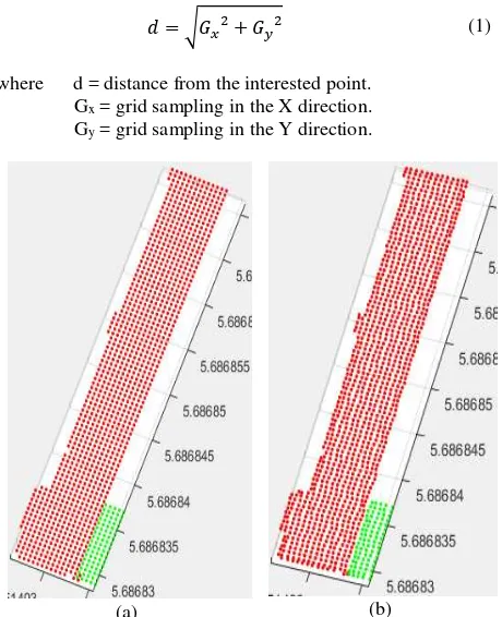
After roof segmentation, edge points of each roof segment are detected. For each roof segment, a regular grid is generated, so that the elevation of points in this grid is equal to the average height of the roof points. The distances between grid points in the x-y directions are calculated from the distance between the roof points, where the distances from each point of the roof points to its closest point are calculated, then the larger distance is selected to be the distance between grid points. These grid points represent the centers of square cells, thus the roof points are located within these cells. Therefore, the 3D means for each cell
are computed, so that all the points located within each cell are detected and then the 3D means of these points are computed. Thus, there are two cases for each cell: (1) 3D regular grid point, (2) 3D mean, and these two sets are related by index. Initially, edge points are detected by grid points, then 3D means by the index are detected as shown in Figure 3.
Figure 2. Roof segmentation.
Now, internal points of the grid are detected and deleted to keep only the edge points. This procedure is done by determining the number of points around each grid point within a distance expressed in equation (1). If the number of points is 8, the interested point is deleted from the grid because it will be inside the roof plane. If the number of points is less than 8, then the point will be edge point. In the last, the detected edge points of the grid are changed with 3D means points (Figure 4).
= √� + � (1)
where d = distance from the interested point. Gx = grid sampling in the X direction. Gy = grid sampling in the Y direction.
(a) (b)
(a) (b)
Figure 4. a) Detected edge points of the grid, b) detected edge points from 3D means points.
2.3 Line approximation
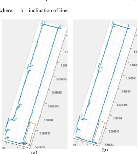
After detection of final edge points, roof lines are approximated. To draw the lines of the buildings, the straight line equation is used. First, the edge points should be grouped so that each group represents a line. For this, initially the edge points are rearranged in the data matrix as in the reality. In other words, each point in the edge points matrix become next to each other. Next, the normals of points are computed. The arranged edge points are grouped based on their adjacent position in the matrix and similarity of directions. Finally, the lines are drawn.
To rearrange the edge points in the matrix data, this process selects the first point in the matrix and finds the nearest point of the matrix and the nearest point is placed next to the first point. This process is repeated for the new point, until all the points are finished. As a result, the matrix of points is rearranged as in the reality. In the next step, (Nx, Ny, Nz) normal of each point is estimated by applying a covariance analysis on three points: the interested point and two nearby edge points. In particular, we solve the eigenvector problem for the covariance matrix:
� =|� | ∑1 − ̅
∈��
− ̅ �
(2)
where Np = the set of points. p = interested point. q = point.
̅: mean of points.
The three eigenvalues are sorted in ascending order, i.e. λ0≤ λ1≤
λ2; and the eigenvector corresponding to the smallest eigenvalue (v0) is the approximated normal at point p (Figure 5a). Nz for all points is zero since the points are located in a horizontal plane. Therefore, angles of directions respecting to the x-axis are estimated by the equation (3). Nx must be positive before using the equation (3), so the normal direction of each point is reversed if Nx < 0. The angles �i are calculated from the X-Axis for using in the straight line equation in the next step, where the angles are in the range [-90, +90]. The angle is positive if its direction is anticlockwise (Ny > 0), and negative if it is clockwise (Ny < 0).
��= �− �� (3)
Next, the edge points are segmented based on their adjacent position in the matrix and similarity of angels. If the angle difference is smaller than the pre-defined threshold, it belongs to a unit segment line. This threshold is about 15 degrees. The final direction of each line must be estimated. The longest line segment is found based on the number of its points, then using equations (2 and 3), its normal vector and angle are estimated by applying a covariance analysis on all line points. This direction is assigned to all parallel lines, then the orthogonal direction is computed (Figure 5b). This method maintains the conditions of orthogonality and parallelism.
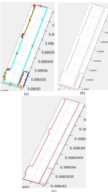
For drawing the lines we need at least one point, so the centroid point for each line is computed as shown in Figure 6a. Next, using centroid points and directions for each line, roof lines are approximated by the straight line equation (4). So that the parameter b is calculated for each line in the equation (4). The lines are approximated and intersections of lines are estimated as displayed in Figure 6b. Finally, regularization constraints must be performed. The main regularization constraints are: (1) merging of lines close to each other, (2) connecting two consecutive parallel lines with an orthogonal line, and (3) intersection of crossover lines. Results are shown in Figure 6c.
= + (4)
where: a = inclination of line.
(a) (b)
(a) (b)
(c)
Figure 6. a) Segmented line points and their centroid points, b) Lines approximation by using the straight line equation, c) Final
edges after applying regularization constraints.
2.4 3D modeling
After extraction of building edges, 3D building models are reconstructed. The floors are flat therefore, for each roof a plane passes through its intersection points of the edge. Using these planes, the roofs are reconstructed. For the modeling of the walls, the adjacent ground points (or the lowest points in the walls points) are detected so that the points are in the neighborhood of building boundaries. Then the lowest elevation of these points is considered as the height of floor. Thus, the roof edges and corners are projected on the building floor. Finally, using the roof edges and the projected edges, the walls are reconstructed as shown in Figure 7.
3. RESULTS AND DISSCUSION
The proposed method has been tested on IEEE sample dataset of the Zeebruges, Belgium study area. The data cover an urban and harbor area in Zeebruges, Belgium. The LiDAR data were captured with Riegl laser scanner. The point density of the LiDAR data is approximately 65 points/m², which is related to point spacing of approximately 10 cm. We selected a building with two roofs and small details in the roof to test the accuracy
of the proposed method, then the proposed method has been applied to other flat buildings. In this research, we focused only on the 3D building modeling, so the building points were already segmented.
(a) (b)
(c)
Figure 7. a) Projected roof edges and corners on the building floor, b) Walls reconstruction, c) 3D flat building modeling
(a) (b)
Figure 8. 3D flat building model with roof points (yellow points), a) top view, b) Lower view.
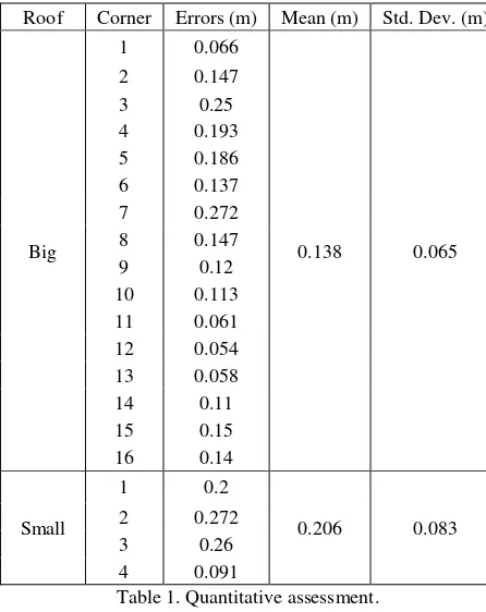
For a more accurate evaluation, a quantitative assessment is performed by digitizing the building roof model manually from LiDAR point clouds. The corners of this model are compared with the corners of the model that has been reconstructed using the proposed method. The results are given in table 1.
Std. Dev. (m) Mean (m)
Errors (m) Corner
Roof
0.065 0.138
0.066 1
Big
0.147 2
0.25 3
0.193 4
0.186 5
0.137 6
0.272 7
0.147 8
0.12 9
0.113 10
0.061 11
0.054 12
0.058 13
0.11 14
0.15 15
0.14 16
0.083 0.206
0.2 1
Small 2 0.272
0.26 3
0.091 4
Table 1. Quantitative assessment.
Table 1 proves that the accuracy of the results is very good. The quality of the 3D model in the big roof is equal approximately to the point density of the LiDAR sensor which is 10 cm. Also, the quality of the 3D model in the small roof is approximately equal to half of the grid spacing which is 40 cm. This is logical because we used 3D mean points to detect the edges. Therefore, the maximum error must be the half. From above, we see that the factors influencing the accuracy of the proposed method are the density of points and the size of the grid spacing. So, the method leads to very good results with good factors. In the end, errors
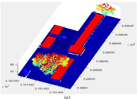
yield from all steps of roof segmentation, edge points detection, line approximation and others. Finally, the proposed method has been applied to other flat buildings as shown in Figure 9.
(a)
(b)
(c)
(e)
Figure 9. a) Point cloud, b) Point cloud of buildings, c) Walls and roofs reconstruction, d) 3D flat buildings modeling, e)
Building models on point cloud.
4. CONCLUSION
There are several factors that affect the accuracy of the final results of 3D building reconstruction of flat roofs in this algorithm. These factors are the nearest neighbor distances, the height difference threshold, the distance between the grid points and the point density. The distance between the grid points is the most important parameter. The algorithm is able to draw the small lines with high accuracy if the distance between the grid points is small. If this distance is big, the small lines that are shorter than the distance, cannot be approximated. As if the distance is a small, gaps within the grid may be formed because the distance between some of the roof points is greater than the distance between the grid points. In the end, this method is very precise for 3D flat building reconstruction from the dense LiDAR point cloud. As we have found that even small details of building have been modeled. This algorithm may have a problem with the buildings including short edges in the low density point cloud, because the distance between the grid points, in this case, will be large and the small lines will be removed
REFERENCES
Arefi, H. and P. Reinartz, 2013. Building reconstruction using DSM and orthorectified images. Remote Sensing 5(4): 1681-1703.
Cheng, L., L. Tong, Y. Chen, W. Zhang, J. Shan, Y. Liu and M. Li, 2013. Integration of LiDAR data and optical multi-view images for 3D reconstruction of building roofs. Optics and Lasers in Engineering 51(4): 493-502.
Elberink, S. O. and G. Vosselman, 2009. Building reconstruction by target based graph matching on incomplete laser data: Analysis and limitations. Sensors 9(8): 6101-6118.
Henn, A., G. Gröger, V. Stroh and L. Plümer, 2013. Model driven reconstruction of roofs from sparse LIDAR point clouds. ISPRS Journal of photogrammetry and remote sensing 76: 17-29.
Lin, H., J. Gao, Y. Zhou, G. Lu, M. Ye, C. Zhang, L. Liu and R. Yang, 2013. Semantic decomposition and reconstruction of residential scenes from LiDAR data. ACM Transactions on Graphics (TOG) 32(4): 66.
Maas, H.G. and G. Vosselman, 1999. Two algorithms for extracting building models from raw laser altimetry data. ISPRS Journal of photogrammetry and remote sensing 54(2): 153-163.
Rau, J.Y. and B.C. Lin, 2011. Automatic roof model reconstruction from ALS data and 2D ground plans based on side projection and the TMR algorithm. ISPRS journal of photogrammetry and remote sensing 66(6): S13-S27.
Rottensteiner, F., 2003. Automatic generation of high-quality building models from lidar data. IEEE Computer Graphics and Applications 23(6): 42-50.
Sajadian, M. and H. Arefi, 2014. a Data Driven Method for Building Reconstruction from LiDAR Point Clouds. The International Archives of Photogrammetry, Remote Sensing and Spatial Information Sciences 40(2): 225.
Tarsha-Kurdi, F., T. Landes, P. Grussenmeyer and M. Koehl, 2007. Model-driven and data-driven approaches using LIDAR data: Analysis and comparison. International Archives of Photogrammetry, Remote Sensing and Spatial Information Sciences 36: 3-W49A.
Vögtle, T. and E. Steinle, 2005. Fusion of 3D building models derived from first and last pulse laserscanning data. Information Fusion 6(4): 275-281.
Wang, H., W. Zhang, Y. Chen, M. Chen and K. Yan, 2015. Semantic decomposition and reconstruction of compound buildings with symmetric roofs from Lidar data and aerial imagery. Remote Sensing 7(10): 13945-1397.
