Directory UMM :Journals:Journal Of Policy Modeling:Vol22.Issue1.2000:

(1)

Mordechai E. Kreinin, Michigan State University

This paper tests the accuracy of annual forecasts made by the OECD and the IMF of: real GDP growth rate, the GDP deflator, unemployment, and the trade balance. These projections are made for each OECD country, and cover a period of about 25 years. Neither the OECD nor the IMF succeed in forecasting cyclical turning points. But other than that, their projections appear fairly robust and certainly superior to those of a “naive” model. 2000 Society for Policy Modeling. Published by Elsevier Science Inc.

Key Words: Unbiased forecast; Real GDP; DGP deflator.

1. INTRODUCTION

Every year and half-year the OECD provides projections of several economic variables, published in the OECD Economic Outlook, while the IMF provides similar projections published in the IMFWorld Economic Outlook. Because these forecasts are used extensively by governmental and nongovernmental organiza-tions, it is useful to examine their accuracy. The assessment pro-vided here differs in approach from earlier assessments,1_{but their}

purpose is similar. Because much previous work concentrated on the IMF projections (see footnote 1), the present effort is devoted mainly to those of the OECD. Whenever possible, a comparison is made between the two. But because of differences in years and countries of coverage (as contained in the IMFpublicly published

1_{See: Smyth, D.J. and Ash, J.C.K. “Forecasting GDP, The Rate of Inflation and the}

Balance of Trade: The OECD Performance”,Economic Journal, June 1975, pp. 361–364; Artis, M.J. “How Accurate Is the World Economic Outlook? A Post Mortem On Short-Term Forecasting at the IMF,” IMF,Staff Studiesfor the World Economic Outlook, July 1988, pp. 1–48. Barrionuevo, J.M. “How Accurate Are the World Economic Outlook Projections?”,Staff Studiesfor the World Economic Outlook, December 1993, pp. 28–45; andIbid, May 1992; and DeMasi, P. “The Difficult Art of Economic Forecasting”Finance and Development, December 1996. See also the literature cited therein.

(2)

version), the comparison is rather imperfect. Finally, the accuracy of projections will be compared with that of a “Naive” forecast. Of the several possible “Naive” forecasts, I have chosen to follow the book of Ecclesiastes (Chapter 1, verse 9):

“That which has been is that which shall be

And that which hath been done is that which shall be done And there is nothing new under the sun.”

In other words, the Naive forecasts assumes that last year’s development (e.g., growth rate or inflation) will be the forecast for the next year.

OECD forecasts are generated by “country desks,” and are based on: models, the desk-official judgment, accounting checks, anticipated shocks, and the like. Each “forecasting round” lasts 3 months, and contains two to three iterations; it begins with exogenous assumptions about exchange rates and other variables. The OECD is restricted to usinggovernmentalprojections of each respective public sector. Estimates are made of each country’s domestic demand and import demand, and a global model is used to check the consistency of a country’s imports with other countries’ exports. That adds to the accuracy of the trade balances projections, as shown in Section 5 below. Consistency of interest rates between countries (and that of other variables) are also checked. Reliance is made on none-OECD sources such as the IMF and the World Bank. In particular, the OECD reads the IMF projections that appear earlier.

2. REAL GDP GROWTH RATES

For each year (t) the OECDEconomic Outlookmakes growth rate projections for every OECD member in the preceding year (t2_{1), where the “forecasting round” is done during September–} November; and in the middle of the year itself (t 2_{1/2), where} the “forecasting round” is done during March–May. The actual growth rate is published in the following year (t11). For example, the projections for 1990 appear in 1989 and then in mid-1990, while the actual 1990 growth rates are published in 1991.

To estimate the accuracy of the projections, the actual growth rate (Ga) is regressed on the “year earlier” (t21) projection and separately on the midyear (t2 _{1/2) projection:}

Ga5a1b Pt211 e Ga5a1b Pt21/21 e (1)

(3)

years and countries combined. Individual country errors can offset each other in the second and third approaches.

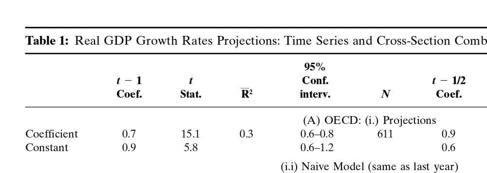
Table 1 presents the regression results for all country–year com-binations. The midyear OECD projections are more accurate than the year-earlier forecasts, but in neither case do the coefficient 1 and the constant zero fall within the 95 percent of their respective confidence intervals. On the other hand, the projections are supe-rior to the results of the “Naive” model. Similarly, the IMF projec-tions appear superior to its corresponding “Naive” model. But the OECD and IMF forecasts are not comparable because they differ both in the number of countries and years of coverage.

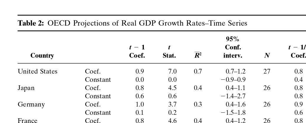
More important are the individual country projections. Those made by the OECD for the eight largest countries are shown in Table 2. For seven of the countries (all except Italy) the year-earlier projections are unbiased in a sense that thedual criterion is met: the coefficient 1 and the constant 0 fall within their respec-tive 95-percent confidence intervals. The U.S. projections appear “best” in terms of the statistical properties. In general, the midyear projections are superior to the year-earlier ones, as might be expected.

In the following smaller countries the coefficient 5 _{1 and the} constant 5 _{0 falls within their respective 95-percent confidence} intervals: Austria, Belgium, Denmark, Finland, Greece, The Neth-erlands, Portugal, Spain, Sweden, Switzerland, and Turkey. Nei-ther condition is met in Norway. Only one of the conditions (coef-ficient51) is met in Iceland, Ireland, and Luxemburg.

In the cross-sectional regressions (not shown) both conditions are met in 15 out of 27 years, but there is no discernible improve-ment over time. Also the midyear projections do not represent a marked improvement over the year-earlier ones.

(4)

M.

E.

[image:4.612.74.574.132.310.2]

Kreinin

Table 1: Real GDP Growth Rates Projections: Time Series and Cross-Section Combined

95% 95%

t21 t Conf. t21/2 t Conf.

Coef. Stat. R2 _interv. N _Coef. _Stat. _R2 _interv. N

(A) OECD: (i.) Projections

Coefficient 0.7 15.1 0.3 0.6–0.8 611 0.9 27.9 0.5 0.83–0.96 644

Constant 0.9 5.8 0.6–1.2 0.6 5.1 0.4–0.9

(i.i) Naive Model (same as last year)

Coefficient 0.4 13.5 0.2 0.3–0.47 893

Constant 2.0 14.7 1.7–2.3

(B) IMF: (i) Projections

Coefficient 0.7 3.1 0.1 0.1–1.1 80 0.6 9.0 0.4 0.5–0.75 112

Constant 0.6 1.0 2_0.6–1.9 _0.9 _4.7 _0.5–1.3

Coefficient 0.4 5.3 0.2 0.3–0.6 112

(5)

OF

OECD

AND

IMF

P

[image:5.612.70.589.115.324.2]

ROJECTION

Table 2: OECD Projections of Real GDP Growth Rates–Time Series

95% 95%

t2₁ t Conf. t2_1/2 t Conf.

Country Coef. Stat. R2 _interv. N _Coef. _Stat. R2 _interv. N

United States Coef. 0.9 7.0 0.7 0.7–1.2 27 0.8 10.0 0.8 0.6–0.9 27

Constant 0.0 0.0 2_0.9–0.9 _0.4 _1.4 2_0.2–1.0

Japan Coef. 0.8 4.5 0.4 0.4–1.1 26 0.8 8.0 0.7 0.6–1.0 28

Constant 0.6 0.6 2_1.4–2.7 _0.8 _1.3 2_0.5–2.1

Germany Coef. 1.0 3.7 0.3 0.4–1.6 26 0.9 9.0 0.7 0.7–1.1 28

Constant 0.1 0.2 2_1.5–1.8 _0.6 _1.7 2_0.1–1.2

France Coef. 0.8 4.6 0.4 0.4–1.2 26 0.8 8.8 0.7 0.6–1.0 28

Constant 0.5 0.8 2_0.7–1.7 _0.7 _2.1 _0.0–1.3

United Kingdom Coef. 0.9 3.7 0.3 0.4–1.4 26 1.1 10.1 0.8 0.9–1.3 28

Constant 0.4 0.6 2_0.8–1.6 _0.4 _1.3 2_0.2–0.9

Canada Coef. 1.4 5.3 0.5 0.8–1.9 26 1.0 7.5 0.7 0.7–1.3 28

Constant 2_1.0 2_1.1 2_2.9–0.8 _0.2 _0.5 2_0.8–1.3

Italy Coef. 0.6 3.6 0.3 0.3–1.0 26 0.9 7.0 0.6 0.6–1.2 28

Constant 1.4 2.2 0.1–2.6 0.7 1.5 2_0.2–1.6

Australia Coef. 0.6 2.0 0.1 2_0.0–1.2 ₂₂ _0.9 _5.0 _0.5 _0.5–1.2 ₂₃

(6)

[image:6.612.56.368.114.316.2]

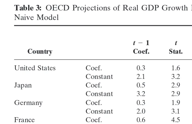
Table 3: OECD Projections of Real GDP Growth Rate–Time Series Naive Model

95%

t21 t Conf.

Country Coef. Stat. R2 _interv. N

United States Coef. 0.3 1.6 0.0 2_0.1–0.6 ₃₄

Constant 2.1 3.2 0.8–3.4

Japan Coef. 0.5 2.9 0.2 0.1–0.8 34

Constant 3.2 2.9 1.0–5.5

Germany Coef. 0.3 1.9 0.1 2_0.0–0.7 ₃₃

Constant 2.0 3.1 0.7–3.3

France Coef. 0.6 4.5 0.4 0.3–0.9 33

Constant 1.2 2.2 0.1–2.4

United Kingdom Coef. 0.3 1.9 0.1 0.0–0.7 33

Constant 1.5 2.9 0.4–2.6

Canada Coef. 0.4 2.5 0.1 0.1–0.7 33

Constant 2.3 3.1 0.8–3.9

Italy Coef. 0.3 2.2 0.1 0.0–0.7 33

Constant 2.1 3.1 0.7–3.5

Australia Coef. 0.3 1.7 0.1 2_0.1–0.6 ₃₃

Constant 2.8 4.0 1.4–4.3

statistical properties are rather poor, but they improve consider-ably in the midyear projections. Yet the dual criterion is met in most cases. In the cross-sectional regressions, with only eight observations, the dual criterion is met in 10 out of 15 years.

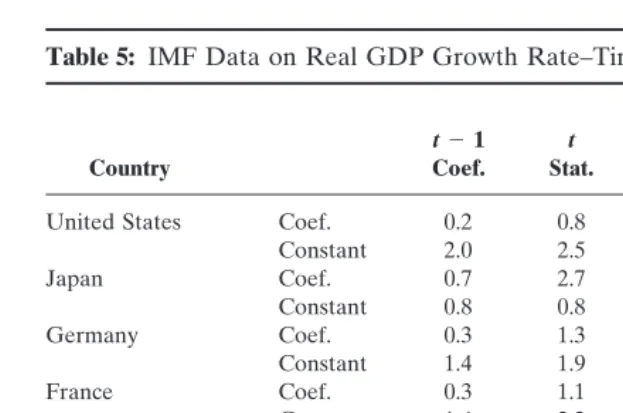
These results are superior to forecast by the Naive model shown in Table 5.

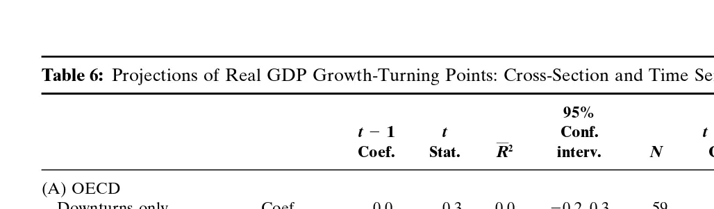
Where the OECD and IMF projections do poorly is in forecast-ing the turnforecast-ing points. Table 6 shows poor statistical properties, and coefficients at variance with expectations. The only possible exception is in the IMF midyear forecast for the downturns and upturns combined.

3. INFLATION

(7)

OF

OECD

AND

IMF

P

[image:7.612.71.588.116.324.2]

ROJECTION

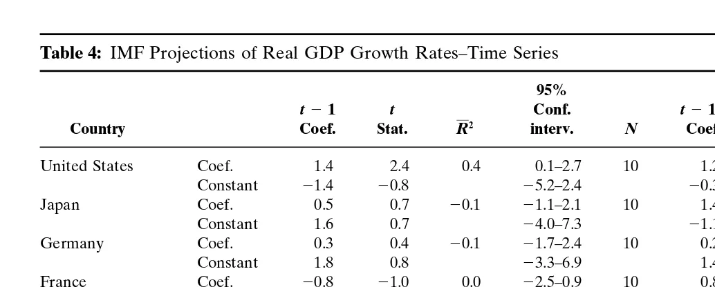
Table 4: IMF Projections of Real GDP Growth Rates–Time Series

95% 95%

t2₁ t Conf. t2_1/2 t Conf.

Constant 2_1.4 2_0.8 2_5.2–2.4 2_0.3 2_0.8 2_1.0–0.4

Japan Coef. 0.5 0.7 2_0.1 2_1.1–2.1 ₁₀ _1.4 _7.3 _0.8 _1.0–1.8 ₁₄

Constant 1.6 0.7 2_4.0–7.3 2_1.1 2_1.7 2_2.5–0.3

Germany Coef. 0.3 0.4 2_0.1 2_1.7–2.4 ₁₀ _0.2 _2.0 _0.2 _0.0–0.4 ₁₄

Constant 1.8 0.8 2_3.3–6.9 _1.4 _2.6 _0.2–2.5

France Coef. 2_0.8 2_1.0 _0.0 2_2.5–0.9 ₁₀ _0.8 _2.3 _0.2 _0.0–1.5 ₁₄

Constant 4.0 2.3 2_0.1–8.1 _0.7 _1.2 2_0.6–1.9

United Kingdom Coef. 2.2 1.9 0.2 2_0.4–4.9 ₁₀ _1.1 _7.9 _0.8 _0.8–1.5 ₁₄

Constant 2_3.1 2_1.1 2_9.8–3.6 _0.6 _1.7 2_0.2–1.2

Canada Coef. 1.4 2.0 0.2 2_0.2–3.0 ₁₀ _1.4 _5.9 _0.7 _0.9–1.9 ₁₄

Constant 2_1.7 2_0.8 2_6.8–3.4 2_0.6 2_1.0 2_2.0–0.8

Italy Coef. 0.5 1.2 0.0 2_0.5–1.5 ₁₀ _0.9 _3.1 _0.4 _0.3–1.5 ₁₄

Constant 0.8 0.7 2_2.0–3.6 _0.4 _0.6 2_0.9–1.6

Other OECD Coef. 2_0.0 2_0.0 2_0.1 2_3.0–3.0 ₁₀ _1.1 _2.1 _0.2 2_0.2–2.2 ₁₄

(8)

[image:8.612.56.368.99.305.2]

Table 5: IMF Data on Real GDP Growth Rate–Time Series Naive Model

95%

t21 t Conf.

United States Coef. 0.2 0.8 0.0 2_0.4–0.8 ₁₄

Constant 2.0 2.5 0.2–3.8

Japan Coef. 0.7 2.7 0.3 0.1–1.2 14

Constant 0.8 0.8 2_1.3–3.0

Germany Coef. 0.3 1.3 0.0 2_0.2–0.9 ₁₄

Constant 1.4 1.9 2_0.2–3.0

France Coef. 0.3 1.1 0.0 2_0.3–0.9 ₁₄

Constant 1.4 2.2 0.0–2.8

Constant 1.1 2.0 2_0.1–2.3

Canada Coef. 0.3 1.0 0.0 2_0.3–0.9 ₁₄

Constant 1.9 1.9 2_0.3–4.0

Italy Coef. 0.4 1.7 0.1 2_0.1–0.9 ₁₄

Constant 1.0 1.8 2_0.2–2.3

Other Europe Coef. 0.5 2.1 0.2 2_0.0–1.1 ₁₄

Constant 1.1 1.7 2_0.3–2.4

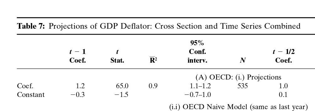
sets of forecasts is impossible by reason of different years and countries of coverage.

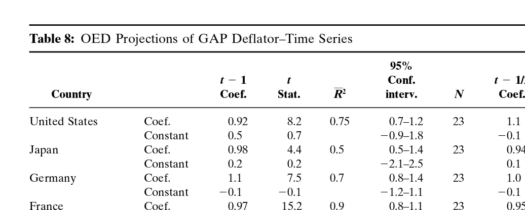
Table 8 shows that the OECD inflation projections for individ-ual countries meet the dindivid-ual criterion (coefficient 5 _{1 and} con-stant5 0 within the respective 95-percent confidence intervals) and have desirable statistical properties. The United States and France exhibit the most robust results. Indeed, the dual criterion is met also in all but two (Greece and Luxembourg) of the small OECD countries, not shown in the tables. The midyear projections constitute an improvement over the year-earlier ones. In the cross-sectional regressions for the years 1975–94, the dual criterion was met in 14 years, while at least one criterion was met in 5 years.

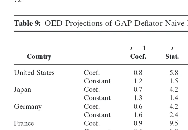
However, as shown in Table 9, the Naive model gives equally unbiased results, for both the large and the small (not shown) OECD countries. In its cross-sectional regressions for 1973–94 the dual criterion was met in 12 years, and at least one of them was not met in 10 years.

(9)

OF

OECD

AND

IMF

P

[image:9.612.70.584.142.293.2]

ROJECTION

Table 6: Projections of Real GDP Growth-Turning Points: Cross-Section and Time Series Combined

95% 95%

t2₁ t _Conf. t2_1/2 t _Conf.

Coef. Stat. R2 _interv. N _Coef. _Stat. R2 _interv. N

(A) OECD

Downturns only Coef. 0.0 0.3 0.0 2_0.2–0.3 ₅₉ _0.4 _3.3 _0.1 _0.1–0.6 ₆₁

Constant 2_1.5 2_4.1 2_2.1–0.8 2_1.3 2_4.6 2_1.8–0.7

Downturns and upturns Coef. 0.2 1.1 0.0 2_0.1–0.5 ₁₁₉ _0.7 _8.0 _0.3 _0.6–0.9 ₁₂₁

combined Constant 0.5 1.5 2_0.1–1.1 _0.2 _0.8 2_0.2–0.6

(B) IMF

Downturns only Coef. 0.7 1.9 0.2 2_0.0–1.4 ₈ _0.3 _2.0 _0.2 _0.0–0.7 ₁₅

Constant 2_2.4 2_3.1 2_3.8–0.9 2_1.0 2_4.2 2_1.5–0.5

Downturns and upturns Coef. 2_0.0 2_0.0 _0.0 2_1.2–1.2 ₁₄ _1.3 _5.6 _0.6 _0.7–1.4 ₂₆

(10)

M.

E.

[image:10.612.73.575.132.310.2]

Kreinin

Table 7: Projections of GDP Deflator: Cross Section and Time Series Combined

95% 95%

t21 t Conf. t21/2 t Conf.

Coef. Stat. R2 _interv. N _Coef. _Stat. _R2 _interv. N

(A) OECD: (i.) Projections

Coef. 1.2 65.0 0.9 1.1–1.2 535 1.0 69.5 0.93 1.0–1.1 563

Constant 2_0.3 2_1.5 2_0.7–1.0 _0.1 _0.9 2_0.2–0.4

(i.i) OECD Naive Model (same as last year)

Coef. 0.9 48.6 0.8 0.9–1.0 608

Constant 0.4 1.3 2_0.2–0.9

(B) IMF: (i) Projections

Coef. 0.9 8.8 0.6 0.7–1.1 80 0.9 30.6 0.9 0.9–1.0 112

Constant 0.6 1.3 2_0.3–1.4 _0.2 _0.8 2_0.3–0.7

Coef. 0.8 25.9 0.9 0.7–0.8 111

(11)

OF

OECD

AND

IMF

P

[image:11.612.71.589.116.324.2]

ROJECTION

Table 8: OED Projections of GAP Deflator–Time Series

95% 95%

t2₁ t Conf. t2_1/2 t Conf.

Constant 0.5 0.7 2_0.9–1.8 2_0.1 2_0.3 2_0.8–0.6

Japan Coef. 0.98 4.4 0.5 0.5–1.4 23 0.94 16.1 0.9 0.8–1.1 26

Constant 0.2 0.2 2_2.1–2.5 _0.1 _0.3 2_0.6–0.9

Germany Coef. 1.1 7.5 0.7 0.8–1.4 23 1.0 16.1 0.9 2_0.9–1.2 ₂₆

Constant 2_0.1 2_0.1 2_1.2–1.1 2_0.1 2_0.2 2_0.6–0.5

France Coef. 0.97 15.2 0.9 0.8–1.1 23 0.95 20.8 0.95 0.9–1.0 26

Constant 0.4 0.9 2_0.6–1.5 _0.4 _1.1 2_0.3–1.1

Constant 0.9 0.7 2_1.6–3.4 _0.5 _1.2 2_0.3–1.3

Canada Coef. 1.1 6.4 0.6 0.7–1.4 23 1.1 12.3 0.9 0.9–1.3 26

Constant 2_0.5 2_0.5 2_2.8–1.8 2_0.5 2_0.8 2_1.6–0.7

Italy Coef. 0.94 10.1 0.8 0.7–1.1 23 0.9 22.2 0.95 0.8–1.0 26

Constant 2.0 1.9 2_0.2–4.2 _1.5 _3.1 _0.5–2.5

Australia Coef. 0.93 5.8 0.6 0.6–1.3 20 0.93 9.5 0.8 0.7–1.1 20

(12)

[image:12.612.56.368.88.305.2]

Table 9: OED Projections of GAP Deflator Naive Model

95%

t21 t Conf.

United States Coef. 0.8 5.8 0.6 0.5–1.0 27

Constant 1.2 1.5 2_0.4–2.8

Japan Coef. 0.7 4.2 0.4 0.3–1.0 27

Constant 1.3 1.4 2_0.6–3.2

Germany Coef. 0.6 4.2 0.4 0.3–0.9 27

Constant 1.6 2.4 0.2–3.0

France Coef. 0.9 9.5 0.8 0.7–1.1 27

Constant 0.6 0.8 2_0.9–2.1

Constant 2.6 1.8 2_0.4–5.7

Canada Coef. 0.8 6.6 0.6 0.6–1.1 27

Constant 0.9 1.1 2_0.8–2.6

Italy Coef. 0.9 10.3 0.8 0.7–1.1 27

Constant 1.1 1.1 2_1.0–3.2

Australia Coef. 0.9 7.5 0.7 0.7–1.2 22

Constant 0.4 0.3 2_1.9–2.7

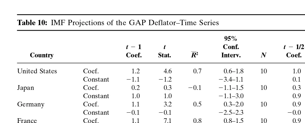
in 9 out of 10 years; and the Naive forecasts gives equally unbiased results (Table 11).

4. UNEMPLOYMENT

Table 12 shows the OECD unemployment projections, where the U.S. results are the “best” of the eight countries, but the dual criterion is met in six of them.2 _{The midyear forecast shows a}

clear improvement over the year-earlier one. However, only in half of the smaller OECD countries was the dual criterion met. In the cross-sectional analysis, the dual criterion was met in 25 out of 27 years. But the Naive model shows equally good if not better results for the eight countries as well as for the small OECD countries (Table 13). Similar observations can be made about the IMF projections (not shown; but available from the author upon request).

5. TRADE BALANCES

Only the OECD and not the IMF provide projections of trade balances. Table 14 shows the combined cross-section and time

(13)

OF

OECD

AND

IMF

P

[image:13.612.71.587.116.324.2]

ROJECTION

Table 10: IMF Projections of the GAP Deflator–Time Series

95% 95%

t2₁ t Conf. t2_1/2 t Conf.

Country Coef. Stat. R2 _Interv. N _Coef. _Stat. R2 _interv. N

Constant 2_1.1 2_1.2 2_3.4–1.1 _0.1 _0.4 2_0.4–0.6

Japan Coef. 0.2 0.3 2_0.1 2_1.1–1.5 ₁₀ _0.3 _2.7 _0.3 _0.1–0.6 ₁₄

Constant 1.0 1.0 2_1.1–3.0 _0.9 _2.7 _0.2–1.6

Germany Coef. 1.1 3.2 0.5 0.3–2.0 10 0.9 6.0 0.7 0.6–1.3 14

Constant 2_0.1 2_0.1 2_2.5–2.3 2_0.0 2_0.0 2_1.3–1.3

France Coef. 1.1 7.1 0.8 0.8–1.5 10 0.9 18.0 0.96 0.8–1.1 14

Constant 2_0.5 2_0.9 2_1.7–0.7 _0.3 _0.8 2_0.5–1.1

Constant 2_1.9 2_0.9 2_7.0–3.2 _0.1 _0.2 2_1.0–1.2

Canada Coef. 0.7 1.6 0.2 2_0.3–1.6 ₁₀ _0.8 _6.0 _0.7 _0.5–1.1 ₁₄

Constant 0.5 0.3 2_2.9–3.9 _0.0 _0.0 2_1.6–1.7

Itlay Coef. 0.6 2.8 0.4 0.1–1.1 10 1.0 16.3 0.95 0.9–1.1 14

Constant 2.7 2.0 2_0.4–5.8 _0.2 _0.3 2_1.3–1.7

Other OECD Coef. 0.1 0.2 2_0.1 2_1.0–1.1 ₁₀ _0.7 _4.9 _0.6 _0.4–1.1 ₁₄

(14)

[image:14.612.60.367.100.305.2]

Table 11: IMF Data on Real GDP Growth Rate–Time Series Naive Model

95%

t21 t Conf.

Constant 0.8 1.1 2_0.7–2.2

Japan Coef. 0.5 2.0 0.2 2_0.4–1.1 ₁₄

Constant 0.6 1.3 2_0.1–1.7

Germany Coef. 0.6 2.5 0.3 0.1–1.1 14

Constant 1.2 1.5 2_0.5–3.0

France Coef. 0.9 12.3 0.9 0.7–1.1 14

Constant 2_0.2 2_0.4 2_1.3–0.9

Constant 2.4 3.5 0.9–3.8

Canada Coef. 0.7 5.9 0.7 0.4–0.9 14

Constant 0.7 1.3 2_0.5–1.9

Italy Coef. 0.8 8.5 0.8 0.6–1.0 14

Constant 0.7 0.6 2_1.7–3.1

Other Coef. 0.9 6.4 0.8 0.6–1.3 14

Europe Constant 2_0.0 2_0.0 2_2.2–2.2

series regressions. The trade balances forecast is shown to be unbiased, with robust statistical properties, and superior to that of the Naive model. The midyear projection is even better. As shown in Tables 15 and 16, the unbiasness exists in the G-5 coun-tries in the time series analysis, and for 11 of the small OECD countries. In the cross-sectional analysis the dual criterion was met in 21 out of 27 years (1967–94). In the Naive model, the dual criterion is met in the G-7 countries and in all the small countries except Turkey. On the other hand, in the cross-sectional analysis the dual criterion was met in only 10 years.

6. CONCLUSION

(15)

OF

OECD

AND

IMF

P

[image:15.612.71.587.116.324.2]

ROJECTION

Table 12: OECD Unemployment Projections–Time Series

95% 95%

t2₁ t Conf. t2_1/2 t Conf.

Constant 0.4 0.5 2_1.3–2.0 _0.4 _1.0 2_0.4–1.2

Japan Coef. 0.6 3.2 0.4 0.2–1.0 13 1.0 11.3 0.9 0.8–1.2 14

Constant 1.0 2.0 2_0.1–2.0 _0.0 _0.0 2_0.5–0.5

Germany Coef. 0.4 3.0 0.4 0.1–0.7 13 0.6 4.6 0.6 0.3–0.8 14

Constant 4.4 4.1 2.0–6.8 3.2 3.5 1.2–5.3

France Coef. 1.0 5.2 0.7 0.6–1.4 13 1.0 11.0 0.9 0.8–1.2 14

Constant 2_0.1 2_0.0 2_4.3–4.2 2_0.2 2_0.2 2_2.1–1.8

Constant 3.9 1.8 2_1.0–8.8 _1.1 _1.1 2_1.1–3.3

Canada Coef. 0.7 3.9 0.5 0.3–1.1 13 0.9 10.9 0.9 0.7–1.1 14

Constant 3.0 1.7 2_0.9–7.0 _1.0 _1.2 2_0.8–2.8

Italy Coef. 0.1 0.7 2_0.0 2_0.3–0.6 ₁₃ _0.9 _6.7 _0.8 _0.6–1.2 ₁₄

Constant 9.5 4.2 4.5–14.5 1.0 0.7 2_2.2–4.2

Australia Coef. 0.8 3.8 0.6 0.3–1.3 11 1.0 16.4 0.96 0.8–1.1 12

(16)

[image:16.612.56.368.99.306.2]

Table 13: OECD Projection of Unemployment–Time Series Naive Model

95%

t21 t Conf.

Constant 1.8 2.3 0.2–3.4

Japan Coef. 0.9 13.0 0.9 0.8–1.1 27

Constant 0.2 1.1 2_0.1–0.5

Germany Coef. 1 18.6 0.9 0.8–1.1 27

Constant 0.3 1.0 2_0.3–0.9

France Coef. 1 29.9 0.9 0.9–1.1 27

Constant 0.4 1.7 2_0.1–0.9

Constant 0.7 1.5 2_0.3–1.7

Canada Coef. 0.9 10.0 0.8 0.7–1.0 27

Constant 1.4 2.0 2_0.1–2.8

Italy Coef. 0.9 22.4 0.9 0.9–1.0 27

Constant 0.6 1.5 2_0.2–1.3

Australia Coef. 0.9 13.4 0.9 0.8–1.1 27

(17)

OF

OECD

AND

IMF

P

[image:17.612.70.586.164.275.2]

ROJECTION

Table 14: OECD Projections of Trade Balances: Cross-Section and Time Series Combined

95% 95%

t2₁ t _Conf. t2_1/2 t _Conf.

Coef. Stat. R2 _interv. N _Coef. _Stat. R2 _interv. N

(i) Projections

Coef. 1.0 62.3 0.9 0.96–1.02 522 1.0 85.9 0.95 0.9–1.0 527

Constant 0.1 0.2 2_0.9–1.2 2_0.8 2_1.6 2_1.8–0.2

(ii) Naive Model

Coef. 1.04 60.6 0.9 1.01–1.07 572

(18)

M.

E.

[image:18.612.70.580.116.324.2]

Kreinin

Table 15: OECD Projections of Trade Balances: Time Series

95% 95%

t2₁ t Conf. t2_1/2 t Conf.

United States Coef. 1.0 18.6 0.9 0.9–1.1 26 1.0 34 0.98 0.97–1.1 23

Constant 2_4.9 2_1.1 2_13–4 2_1.1 2_0.5 2_6.0–3.6

Japan Coef. 1.0 15.3 0.9 0.9–1.1 26 1.0 32.2 0.97 0.93–1.05 23

Constant 2.6 0.6 2_5.9–11.1 _0.8 _0.4 2_3.2–4.8

Germany Coef. 0.8 7.8 0.7 0.6–1.0 26 0.9 13.5 0.9 0.7–1.0 23

Constant 5.4 1.4 2_2.5–13.3 _1.2 _0.5 2_3.7–6.3

France Coef. 0.7 5.1 0.5 0.4–0.9 26 0.9 8.2 0.7 0.7–1.1 28

Constant 2_1.4 2_1.4 2_3.4–0.6 2_1.1 2_1.6 2_2.5–0.3

United Kingdom Coef. 0.9 10 0.8 0.7–1.1 26 0.9 8.9 0.7 0.7–1.1 28

Constant 2_1.5 2_1.0 2_4.4–1.5 2_0.8 2_0.5 2_4.0–2.4

Canada Coef. 0.5 4.3 0.4 0.3–0.8 26 0.7 7.4 0.7 0.5–0.9 28

Constant 2.6 2.4 0.3–5.0 1.8 2.3 0.2–3.4

Italy Coef. 0.5 4.2 0.4 0.3–0.8 26 0.9 7.9 0.7 0.7–1.1 28

Constant 0.9 0.5 2_2.5–4.3 _0.9 _0.9 2_1.3–3.2

Australia Coef. 0.3 1.3 0.0 2_0.1–0.8 ₁₉ _0.6 _3.5 _0.4 _0.3–1.0 ₁₈

(19)

95%

t21 t Conf.

Country Coef. Stat. R2 _Interv. N

Constant 2_6.2 2_1.2 2_1.6–4.0

Japan Coef. 1.0 17.0 0.9 0.9–1.2 28

Constant 3.5 1.0 2_3.7–10.8

Germany Coef. 0.8 7.8 0.7 0.6–1.1 28

Constant 5.8 1.6 2_1.6–13.1

France Coef. 0.8 4.9 0.5 0.4–1.1 28

Constant 0.5 0.5 2_2.7–1.6

Constant 2_1.9 2_1.2 2_5.0–1.2

Canada Coef. 0.8 7.3 0.7 0.6–1.1 28

Constant 1.4 1.7 2_0.3–3.1

Italy Coef. 0.9 5.1 0.5 0.6–1.3 28

Constant 1.2 0.8 2_1.7–4.1

Australia Coef. 0.4 1.5 0.1 2_0.1–0.9 ₂₀

[image:19.612.60.367.101.305.2]