Operations Research Letters 26 (2000) 155–158
www.elsevier.com/locate/dsw
A fast algorithm for the transient reward distribution in
continuous-time Markov chains
H.C. Tijms
a;∗, R. Veldman
baDepartment of Econometrics, Vrije Universiteit, De Boelelaan, 1081 HV Amsterdam, The Netherlands bORTEC Consultants, P.O. Box 490, 2800 AL Gouda, The Netherlands
Received 1 July 1998; received in revised form 1 November 1999
Abstract
This note presents a generally applicable discretization method for computing the transient distribution of the cumulative reward in a continuous-time Markov chain. A key feature of the algorithm is an error estimate for speeding up the calculations. The algorithm is easy to program and is numerically stable. c2000 Elsevier Science B.V. All rights reserved.
Keywords:Transient reward distribution; Discretization algorithm
1. Introduction
A fundamental and practically important problem is the calculation of the transient probability distri-bution of the cumulative reward in a continuous-time Markov chain. Practical applications include computer systems and oil-production platforms with guaranteed levels of performability over nite time periods. In such systems high penalties must be paid when not meeting the guaranteed levels of performability over the specied time interval and thus the computation of the probability of not meeting the performability re-quirement becomes necessary. More specically, con-sider a continuous-time Markov chain {X(t); t¿0} with nite state space I and innitesimal transition ratesqij; j6=i. A reward at rateriis earned for each
∗Corresponding author.
unit of time the system is in statei. Dening the ran-dom variable O(t) by
O(t) = the cumulative reward earned up to timet;
the problem is to calculate the transient reward distri-butionP{O(t)¿ x}for given value of t. An impor-tant special case of this general problem is the case in which the state space I splits up in two disjoint setsIo andIf of operational and failed states and the
reward functionri= 1 fori∈Io andri= 0 fori∈If.
In this case, the transient distribution of the cumula-tive reward reduces to the transient distribution of the cumulative operational time. A transparent and ele-gant algorithm for the 0 –1 reward case was given in De Souza e Silva and Gail [1] using the well-known idea of uniformization in continuous-time Markov chains. Recently, De Souza e Silva and Gail [2] ex-tended their algorithm for the 0 –1 case to the case of general reward rates. Unfortunately, this generalized
156 H.C. Tijms, R. Veldman / Operations Research Letters 26 (2000) 155–158
algorithm is quite complicated and, worse, it is not always numerically stable so its numerical answers may be unreliable. In this note, we present an alter-native algorithm that is both easy to program and numerically stable. This alternative algorithm is based upon discretization. The discretization algorithm it-self is a direct generalization of an earlier algorithm proposed by Goyal and Tantawi [3] for the 0 –1 case. However, we could considerably speed up this naive discretization algorithm by using a remarkably sim-ple estimate for the error made in the discretization. The discretization method has the additional advan-tage of being directly extendable to continuous-time Markov chains with time-dependent transition rates.
2. The discretization algorithm
Let us rst dene fi(t; x) as the joint probability
density of the cumulative reward O(t) up to time t
and the stateX(t) of the process at time t. In other
In the sequel, it is assumed that the reward rates
ri are nonnegative integers. It is no restriction to
make this assumption. Next, we discretize x and t
in multiples of , where is chosen suciently small (i.e. the probability of more than one state transition during a time period should be small). For xed ¿0, the probability density fi(t; x) is
approximated by a discretized function f
i (t; x). In
view of the probabilistic interpretation offi(t; x)x,
this discretized function is dened by the recursion scheme
where{i; i∈I}denotes the probability distribution
of the starting state at time 0. Using the simple-minded approximation
The computational complexity of this algorithm is O(|Nt(t−x)|=2) where N denotes the number of states. In practical applications, one is usually inter-ested inP{O(t)¿ x} forxsuciently close tormaxt
The advantage of this representation is that it requires fewer function evaluations of f
i (u; y). For xed x
and t, the computational eort of the algorithm is proportional to 1=2 and so it quadruples whenis
halved. Thus, the computation time of the algorithm gets very large when the probability P{O(t)¿ x}
is desired in a high accuracy. Another drawback is that no estimate is given for the discretization error. Fortunately, both diculties can be overcome. De-note byP() the right-hand side of (1) (or (2)), and let e() be the dierence between the exact value of P{O(t)¿ x} and the approximate value P(). The following remarkable result was empirically found:
e()≈P()−P(2); (3) when is not too large. In other words, the esti-mateP() of the true value ofP{O(t)¿ x}is much improved when it is replaced by
˜
H.C. Tijms, R. Veldman / Operations Research Letters 26 (2000) 155–158 157 Table 1
Numerical results for the rst example
t= 75; x= 178 t= 75; x= 191
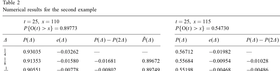
Numerical results for the second example
t= 25; x= 110 t= 25; x= 115
We could not nd in the literature on partial dierential equations a result covering (3) nei-ther we could prove (3) directly. However, on the basis of numerous examples tested, it is our conjecture that e()∼P() − P(2) for
→0.
The numerical results in Tables 1 and 2 demon-strate convincingly that replacing P() by ˜P() =
P() + (P() − P(2)) leads to great improve-ments in accuracy and thus to considerable reduc-tions in computation times. Table 1 refers to a production-reliability system with three operating units and a single repairman. The operation time of each unit is exponentially distributed with mean 1= = 10 and the repair time of any failed unit is exponentially distributed with mean 1= = 1. The repairman can repair only one unit at a time. The system earns a reward at rate ri=i for each unit of
time that i units are in operation. The system starts with all units in good condition. This example can be formulated as a continuous-time Markov chain with state space I ={0;1;2;3}, where state i means that
i units are in operation. The innitesimal transition rates are given byqi; i−1=iandqi; i+1=. In Table
2 we give some results for a second example dealing with a continuous-time Markov chain with state space
I ={1;2;3;4;5}, initial state i = 1, reward vector
Remark. The discretization algorithm needs only a minor modication when in addition to the reward ratesri a xed jump rewardFki is earned each time
158 H.C. Tijms, R. Veldman / Operations Research Letters 26 (2000) 155–158
We found empirically that the error estimate for speed-ing up the convergence also applies in the case with xed jump rewards.
References
[1] E. de Souza e Silva, H.R. Gail, Calculating cumulative operational time distributions of repairable computer systems, IEEE Trans. Comput. 35 (1986) 322–332.
[2] E. de Souza e Silva, H.R. Gail, An algorithm to calculate transient distributions of cumulative rate and impulse rate based rewards, Stochastic Models 14 (1998) 509–536.