DOI 10.1007/s10845-013-0826-y
Optimization of injection-molded light guide plate with
microstructures by using reciprocal comparisons
Chung-Feng Jeffrey Kuo · Gunawan Dewantoro · Chung-Ching Huang
Received: 30 April 2013 / Accepted: 6 August 2013 © Springer Science+Business Media New York 2013
Abstract Injection molding is considered as an effective way to manufacture light guide plate (LGP) with microstruc-tures. However, the determination of processing parame-ters has always been difficult pertaining to shrinkage and warpage, bringing about variations in quality of the injec-tion molded product. This study proposed a procedure for solving the optimization problem utilizing reciprocal com-parisons in data envelopment analysis. This method attempts to improve the comparisons of efficiency between differ-ent systems (CEBDS) which has been done in other works. The objectives are to make the depth and angle of the V-cut microstructures as close to the target values as pos-sible, and make the residual stresses of light guide plate minimum. First, Taguchi method with orthogonal array L18 was applied to reduce the number of experiments. Then, the significant factors which have profound effect to the qual-ity characteristics were confirmed using the ANOVA and main effect analysis. Next, CEBDS and reciprocal compar-isons were conducted to optimize the multi-parameter com-bination. The results were compared and investigated both
C.-F. J. Kuo (
B
)Graduate Institute of Automation and Control, National Taiwan University of Science and Technology, No. 43, Section 4, Keelung Road, Taipei 106, Taiwan, Republic of China e-mail: [email protected]
G. Dewantoro
Department of Electronic and Computer Engineering, Satya Wacana Christian University, 52-60 Diponegoro Street, Salatiga 50711, Indonesia
e-mail: [email protected] C.-C. Huang
Department of Mold and Die Engineering, National Kaohsiung University of Applied Science, 415 Chien Kung Road, Kaohsiung 807, Taiwan, Republic of China
e-mail: [email protected]
theoretically and experimentally. The reproducibility of the experiment was verified by confirming a confidence inter-val of 95 %. It is inferred that the reciprocal comparisons approach is far superior to the CEBDS approach. The results also demonstrated improvements of LGP qualities compared to the best achieved in Taguchi orthogonal array experiment.
Keywords Injection molding·Taguchi method· Reciprocal comparisons·Optimization
Introduction
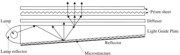
Fig. 1 Backlight unit module
the light guide plate to become distorted (Kazmer 2007;
Umbrello et al. 2010;Bociaga et al. 2010). However, the spec-ification and setting of processing parameters has always pos-sessed difficulties related to shrinkage and warpage, causing variations in quality of the injection molded product. There-fore, processing parameters that minimize thermal-induced residual stress are to be sought, thereby deformed wedge-shaped light guide plate can be avoided. In addition to that, V-cut microstructures, with the target depth of 2.887µm and target angle of 120◦, are kept to be as close to the targets as possible. Thus, the V-cut depth, angle, and residual stress were chosen to be the objectives in this study. Faced with so many processing parameters, relevant research in the past had been trying to discover the relationship between the parame-ters and mold product quality.Choi and Im(1999) analyzed the shrinkage and warpage of the final injection product using numerical analysis method, taking the residual stress issues in the packing pressure and cooling stages into considera-tion, and proving through the residual stress curve that the packing pressure stage had the most profound effect on the results of injection molding. Using Taguchi method, together with nominally-the-best (type II) quality characteristic, Dra-gan et al.(2013) also showed that packing pressure was the most influential process parameters affecting post-molding shrinkage.
L9orthogonal array from the Taguchi method can be car-ried out to investigate the sintering characteristics of Ti-6Al-4V/HA tensile bars (Thian et al. 2002). Its final product was produced using powder injection molding. The processing parameters that were looked into include sintering temper-ature, heating rate, packing time, and cooling rate. From the experimental result, sintering temperature had the most significant effect on sintering characteristics, which is also confirmed byShye et al.(2013). Meanwhile, some research observed that mold temperature is the most important para-meter in injection molding process (Murakami et al. 2008;
Huang et al. 2009;Yun et al. 2013). They showed that high mold temperature had been proven to significantly improve the level of filling with melt plastics in microinjection mold-ing and conducive to the moldmold-ing of microstructures. Accord-ing toSanchez et al.(2012), cooling time was found to be the most significant parameter to reduce warpage, as shown in cases of the box and plastic glass.Guilong et al.(2013)
studied the effects of cavity surface temperature in rapid heat cycle molding on mechanical strength of the molded speci-mens with and without a weld line. From the point of view tensile strength and impact strength, cavity surface tempera-ture was found to be the utmost important parameters.
While the Taguchi method is mainly used for optimiz-ing soptimiz-ingle quality property (Nik and Shahrul 2011;Nor et al. 2010;Hasan et al. 2007), optimal processing parameters that determine the single quality usually do not represent the optimization of process parameters for the overall quality. For this reason, Taguchi method can also be combined with other methods, such as principal component analysis as in
Anthony (2000),Saurav et al. (2009),Humberstone et al.
(2012). Nevertheless, when more than one principal com-ponent, how to trade off to select the solution is unknown. Analytic Hierarchical Process (AHP) with Taguchi method were combined to obtain the optimal multi-parameter of laser scribing system for micro crystalline silicon thin film solar cell isolation and plastic injection molding (Kuo et al. 2010;
Faisal et al. 2013). However, AHP incorporates a priori infor-mation about the response weight that increases uncertainty in the decision-making process. Grey relational analysis was employed in multi-objective optimization by using Taguchi design of experiments (Yang et al. 2012;Kuo et al. 2011;Lin 2012), where the relative significance of processing parame-ters were still required to be known so that the optimal com-binations of the processing parameters levels can be sought. Response Surface Methodology was also used to determine interactions among the control factors (Cicek et al. 2013;
Muhammad et al. 2012). The predictive quadratic models were derived by the RSM to obtain the optimal responses as a function of the parameters.Abbas and Mohammad(2011),
Abbas(2009) studied, respectively, the benevolent formula and comparisons of efficiency between different systems (CEBDS) technique in Data Envelopment Analysis (DEA). The CEBDS technique turns out to be an efficient approach for optimizing process performance with categorical data. However, there was no confirmation experiment to prove the reliability of the results.
experimental
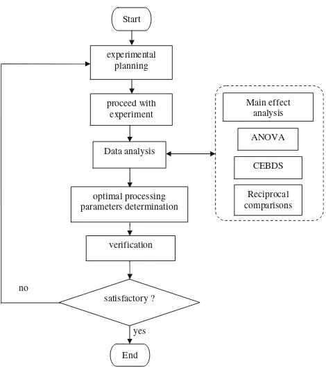
Fig. 2 Flowchart of experimental procedure
and the computational time was reduced. First, Taguchi method with orthogonal array L18 was applied to reduce the number of experiments. Then, the significant factors which have profound effect to the quality characteristics were confirmed using the ANOVA and main effect analysis. Next, CEBDS and reciprocal comparisons were conducted to optimize the multi-parameter combination. The results were compared and investigated both theoretically and experimen-tally. That is, the S/N ratios were predicted under the opti-mal conditions by addition to investigate the total anticipated improvement and the confirmation experiments were carried to verify reproducibility and feasibility through the proposed approach.
Experimentation
The whole experimental procedure of this study is described in Fig.2:
Experimentation plan
The final selection of control factors and their levels is shown in Table1. Eighteen sets of experiments were then conducted as planned by the orthogonal array, with each set of experi-ments repeated four times which means there would be a total of 72 data for each quality characteristic. Four dashed lines were followed by using surface-profile measuring system to measure the depth and angle of molded light guide plates in
Table 1 Eight control factors and their levels for injection molding machine
D. Injection speed (mm/s) 165 180 195
E. Injection pressure (MPa) 220 240 260
F. Packing pressure (MPa) 90 100 110
G. Packing switching (mm) 5 10 15
H. Packing time (s) 1 2 3
order to comprehend the variance of the molded light guide plates.
Material and equipments
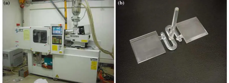
The mold tooling was provided by Plastic Precision Mold-ing Laboratory, Department of Mold and Die EngineerMold-ing, National Kaohsiung University of Applied Science, as shown in Fig. 3. The resin material used for injection molding was optical grade polymethyl methaacrylate (PMMA) with refractive index of 1.49, produced by Japan’s KURARAY Co., Ltd. The injection molding machine was manufactured by Sodick Plustech Co., Ltd. (Model Sodick TR30EH) as shown in Fig.4a. The light guide plate produced by the injec-tion molding process is shown in Fig.4b. The surface profile measuring system used for measuring the light guide plate V-cut measurements is the Form Talysurf PGI 635, made by Taylor Hobson Co., Ltd, as shown in Fig.5a, whilst the resid-ual stress measuring instrument is VML 250P, made by 3D Family Tech. Co., Ltd. as shown in Fig.5b.
Reciprocal comparisons in data envelopment analysis
Data Envelopment Analysis (DEA) is linear programming for measuring the productive efficiency of Decision-Making Units (DMUs) without requiring prescribed weights attached to the multiple inputs and multiple outputs, as described in
Cooper et al.(2006). This proposed reciprocal comparisons method seeks the opportunity to improve CEBDS in DEA which was introduced by Abbas(2009). Here, each DMU is compared in reciprocal manner. That is, for each pair of group, each DMU of one group is evaluated with respect to the DMUs of the opposite group and vice versa. Therefore, for a total of K groups, there will be K!/(2!x(K−2)!) recipro-cal comparisons. Thisinter-comparison, as opposed tointer
dis-Fig. 3 Moving mold-half (left) and fixed mold-half (right)
Fig. 4 aSodick Plustech injection molding machine.bLight guide plate
crimination between two groups. For example, let DMUa
be a random DMU of group 1 to be evaluated, and Ea,2 denotes the efficiency of DMUa with respect to the DMUs
of group 2. ThenEa,2is obtained by solving the following model:
where xa and ya are the input and output vectors for
DMUa,xjandyjare the input and output vectors for DMUs
of group 2. The objective of the linear programming is to adjust the value ofλjsuch thatθis minimum. The efficiency
of each DMU of group 2 with respect to DMUs in group 1 can be easily obtained in a similar manner.
Results and discussion
Taguchi experimental method (Ross 1996)
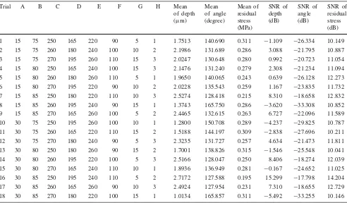
The experimental data of the V-cut depth, V-cut angle, and the residual stress are shown in Table2. On the basis of the S/N ratio available in Table2, main effect analysis was adopted in this study to figure out the main effect of each factor level and the response graphs could be prepared, as shown in Fig.6. From the response graphs, the optimal factor combination for single quality characteristic could be obtained.
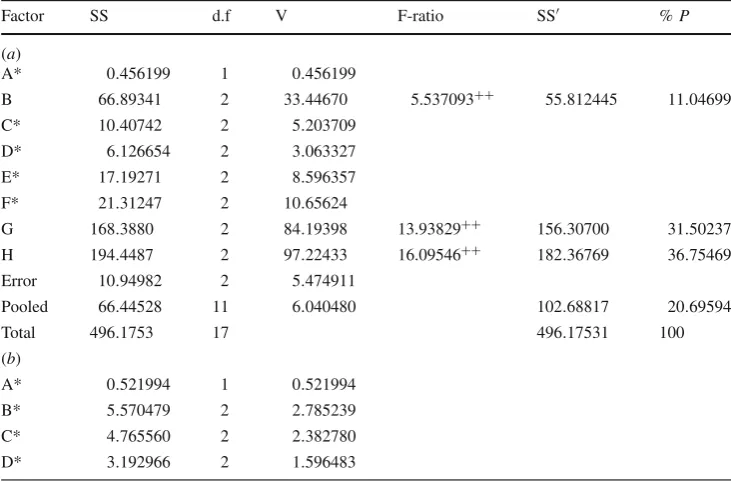
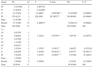
In order to identify the control factors that have signif-icant effects, analysis of variance (ANOVA) for S/N ratio is performed at a certain confidence level. The results of ANOVA for V-cut depth, angle, and residual stress are shown in Table3. From ANOVA of V-cut depth as shown in Table3a, control factors B, G, and H all possess F-ratio greater than that obtained from table of F value with 95 % confidence level. Therefore, all of these factors are significant factors whose effects are strongly believed to be profound. From ANOVA of angle as shown in Table3b, control factors G, and H all possess F-ratio greater than that obtained from table ofFvalue with 95 % confidence level. Therefore, all of these factors are significant factors whose effects are strongly believed to be profound. From ANOVA of residual stress as shown in Table3c, control factors B, G, and H all possess
Table 2 The orthogonal array with the averages and SN ratios of all qualities
Trial A B C D E F G H Mean
2 15 75 260 180 240 100 10 2 2.1986 131.689 0.286 3.088 −21.795 10.887
3 15 75 270 195 260 110 15 3 2.0247 130.648 0.280 0.992 −20.723 11.054
4 15 80 250 165 240 100 15 3 2.1476 131.240 0.279 2.308 −21.234 11.094
5 15 80 260 180 260 110 5 1 1.9650 140.065 0.243 0.639 −26.128 12.273
6 15 80 270 195 220 90 10 2 2.0228 135.543 0.259 1.167 −23.835 11.732
7 15 85 250 180 220 110 10 3 2.5274 128.418 0.215 8.310 −18.658 12.832
8 15 85 260 195 240 90 15 1 1.3743 165.750 0.286 −3.620 −33.308 10.852
9 15 85 270 165 260 100 5 2 2.4465 132.615 0.263 6.727 −22.096 11.589
10 30 75 250 195 260 100 10 1 1.2800 150.708 0.289 −4.237 −29.825 10.787
11 30 75 260 165 220 110 15 2 1.5188 144.197 0.309 −2.838 −27.696 10.211
12 30 75 270 180 240 90 5 3 2.3235 131.727 0.257 4.634 −21.473 11.811
13 30 80 250 180 260 90 15 2 1.7001 138.826 0.315 −1.546 −25.548 10.041
14 30 80 260 195 220 100 5 3 2.5166 128.047 0.250 8.406 −18.274 12.039
15 30 80 270 165 240 110 10 1 1.8936 136.949 0.281 −0.167 −24.652 11.025
16 30 85 250 195 240 110 5 2 2.7172 127.588 0.195 15.299 −17.798 14.204
17 30 85 260 165 260 90 10 3 2.4924 127.954 0.231 7.310 −18.655 12.729
Fig. 6 The response graph foraV-cut depthbV-cut anglecresidual stress
Table 3 ANOVA results for (a) V-cut depth (b) V-cut angle (c) residual stress
Factor SS d.f V F-ratio SS′ %P
(a)
A* 0.456199 1 0.456199
B 66.89341 2 33.44670 5.537093++ 55.812445 11.04699
C* 10.40742 2 5.203709
D* 6.126654 2 3.063327
E* 17.19271 2 8.596357
F* 21.31247 2 10.65624
G 168.3880 2 84.19398 13.93829++ 156.30700 31.50237
H 194.4487 2 97.22433 16.09546++ 182.36769 36.75469
Error 10.94982 2 5.474911
Pooled 66.44528 11 6.040480 102.68817 20.69594
Total 496.1753 17 496.17531 100
(b)
A* 0.521994 1 0.521994
B* 5.570479 2 2.785239
C* 4.765560 2 2.382780
Table 3 continued
∗
Pool-up terms
++
Significant factor at 95 % CI
+
Significant factor at 90 % CI
Factor SS d.f V F-ratio SS′ %P
E* 5.215428 2 2.607714
F* 17.02818 2 8.514089
G 83.37654 2 41.68827 9.456388++ 74.559587 18.90894
H 253.6219 2 126.8109 28.76525++ 244.80493 62.08460
Error 21.01560 2
Pooled 57.31020 13 4.408477 74.944113 19.00646
Total 394.3086 17 394.30863 100
(c)
A* 0.01555 1
B 4.64842 2 2.32421 5.87759++ 3.85755 18.49752
C* 0.31918 2
D* 1.31109 2
E* 0.63673 2
F 2.47414 2 1.23707 3.12837+ 1.68327 8.071516
G 6.82858 2 3.41429 8.63424++ 6.03771 28.95173
H 3.34434 2 1.67217 4.22867++ 2.55346 12.24425
Error 1.27636 2
Pooled 3.55892 9 0.39544 6.72241 32.23499
Total 20.8544 17 20.85440 100
F-ratio greater than that obtained from table ofFvalue with 95 % confidence level, whereas control factor F possesses F-ratio greater than that obtained from table ofF value with 90 % confidence level. Therefore, all of these factors are sig-nificant factors whose effects are strongly believed to be pro-found. By combining ANOVA and main effect analysis, one can achieve the optimal parameters combination for the V-cut depth that is B3,G1, and H3; where mold temperature is 85◦C, packing switching is 5 mm, and the packing time is 3 s. Meanwhile, the optimal parameters combination for the V-cut angle is G1and H3. Lastly, the optimal parameters combination for the residual stress is B3,F3,G1, and H3.
Optimization in Taguchi orthogonal array
All trials in Taguchi’s orthogonal array turn out to be DMU with the multi-objective as the inputs and outputs for all DMUs. In this research, there are 18 experiments in Taguchi’s orthogonal array of 8 factors with 3 responses. Here, both CEBDS and reciprocal comparisons are investi-gated to demonstrate the improvement of the latter method. The procedure is outlined in following steps:
Step 1. Trial j (j = 1, . . .,18) shown in Table 2
are considered as DMUj. The relative efficiency of DMUj, which is calculated as the ratio of the sum of the weighted outputs relative to the sum of weighted inputs, is improved when the sum of weighted outputs is increased and/or the sum of the weighted inputs is
decreased. Since all of S/N ratios are larger-the-better type, in consequence, set all of the responses as outputs, which are preferred at maximum, and set a unit (one) as the input.
Step2. Normalize the S/N ratio,Xi j, for the jth response
at theith trial.Xi j is now normalized asZi j, which lies
between 0 and 1, by the following formula, to avoid the effect of adopting different units. The result is shown in Table4. It is obvious that trial 16 is the most superior among all trials in Taguchi orthogonal array experimen-tation set.
Zi j =
Xi j−min
Xi j,i=1, . . . ,m
max
Xi j,i=1, . . . ,m−minXi j,i=1, . . . ,m
for i=1, . . . ,m, j=1, . . . ,n (2)
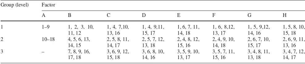
Step3. For each factor in Table2, the 18 DMUs are then separated into groups, each at the same factor level, as shown in Table5. In this case, factor A is assigned at two levels; A1 and A2. As a result, the 18 DMUs for factor A are divided into two groups each of 9 DMUs.
Step 4.For each of the factors A to H, the efficiencies
Table 4 Normalized S/N ratio
(dB) Trial no. Depth Angle Stress Trial no. Depth Angle Stress
1 0.2108 0.4496 0.3353 10 0.0604 0.2245 0.2876
2 0.4127 0.7423 0.0223 11 0.1277 0.3618 0.1177
3 0.3119 0.8114 0.0717 12 0.4870 0.7631 0.0000
4 0.3752 0.7784 0.0834 13 0.1898 0.5003 0.0675
5 0.2949 0.4629 0.7257 14 0.6685 0.9693 0.0673
6 0.3203 0.6108 0.2715 15 0.2561 0.5581 0.0631
7 0.6639 0.9445 0.3009 16 1.0000 1.0000 1.0000
8 0.0900 0.0000 0.0121 17 0.6158 0.9447 0.8600
9 0.5877 0.7229 0.2293 18 0.0000 0.0034 0.1574
Table 5 The index of DMU that belong to groups of each factor Group (level) Factor
efficiency,E1,1of DMU1with respect to the 6 DMUS of group 1 is obtained by solving the following model:
E1,1= minθ
TheE1,1is measured as 1.000.
Similarly, the efficiency of DMU1 with respect to the six DMUs of group 2,E1,2, is obtained by solving the following model:
TheE1,2is evaluated as 0.693.
0.4496≤
The optimal efficiency of DMU1,E1, is then decided as
0.45; which is the minimum of {1.000, 0.693, 0.45}. The
E2 to E18 for DMU2 to DMU18 are evaluated in a sim-ilar manner. The Ej values for the 18 DMUs using the
CEBDS approach for the rest of the factors are obtained similarly.
Step 5.The level efficiency is calculated as the average
of theEj values measured using CEBDS approach for
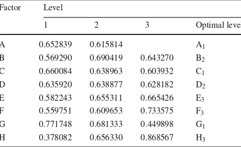
the DMUs at that factor level. Table6displays the cal-culated efficiencies of all factor levels. For illustration, the efficiency of B1, 0.56929, is calculated as the sum of the efficiencies for the six DMUs at level 1 divided by six. Similarly, the efficiency for B2and B3are calcu-lated as 0.690419 and 0.64327, respectively. Obviously, the largest level efficiency for factor B corresponds to B2, and hence, the optimal level of factor B is selected at
Table 6 The level of efficiency using the CEBDS approach Factor Level
1 2 3 Optimal level
A 0.652839 0.615814 A1
B 0.569290 0.690419 0.643270 B2 C 0.660084 0.638963 0.603932 C1 D 0.635920 0.638877 0.628182 D2 E 0.582243 0.655311 0.665426 E3 F 0.559751 0.609653 0.733575 F3 G 0.771748 0.681333 0.449898 G1 H 0.378082 0.656330 0.868567 H3
B2. In a similar manner, the optimal levels for the other factors are decided at A1,C1,D2,E3,F3,G1,H3.
Step6. Reciprocal comparisons solve the problem in the same way as that of CEBDS. However, unlike CEBDS, each DMU is only evaluated based onintergroup compar-ison rather than bothinter-andwithin-group. Therefore, comparison between group 2 and group 2 (within-group comparison) is not required. For example, one does not need to solveE4,2,E5,2,E6,2,E13,2,E14,2,E15,2for fac-tor B because DMU4,DMU5,DMU6,DMU13,DMU14, and DMU15belong to group 2 in factor B. This step is repeated until the reciprocal comparison efficiencies of 18 DMUs for all factors are obtained.
Step 7. The efficiency is calculated as the average of
theEj,kvalues evaluated by the reciprocal comparisons
approach at that factor level, as shown in Table7. For illustration, the efficiency of B1, 1.485, is calculated as the average ofEj,1 values. Similarly, the efficiency for B2and B3are calculated as 0.86 and 0.63, respectively. The minimum of {1.485, 0.86, and 0.63} corresponds to B3, and hence, the optimal level of factor B is decided at B3. In a similar way, the optimal levels for factors A to H are decided at A2,B3,C1,D3,E2,F3,G1, and H3, respectively.
Confirmation experiments
After the optimum light guide plate processing parame-ters was obtained through both approaches, the confirmation experiments were conducted.
Verification of CEBDS approach
Take the V-cut depth for instance, the S/N ratio of optimal processing parameters is:
ˆ
S N =T +(B2−T)+(G1−T)+(H3−T)
= B2+G1+H3−2T
Table 7 The level of efficiency using the reciprocal comparisons
DMUj Factor
A B C D
Ej,1 Ej,2 Ej,1 Ej,2 Ej,3 Ej,1 Ej,2 Ej,3 Ej,1 Ej,2 Ej,3
Average 0.833 0.65 1.485 0.86 0.63 0.62 0.721 1.471 0.744 0.834 0.64
Optimal level A2 B3 C1 D3
DMUj E F G H
Average 1.165 0.62 0.719 0.795 1.384 0.585 0.57 0.711 2.93 1.729 0.623 0.61
=1.801199+5.765991+5.326707−2×2.215056
=8.463784 dB (6)
where T is the total average value of S/N ratio; B2,G1and H3 are the average of the S/N ratio for those factor level. Confidence Interval (CI) of theoretically-predicted value is calculated:
C I1=
Fα;1,v2×Verr or×
1
ne f f
=
4.84×6.04048× 7
18 =3.371962d B (7)
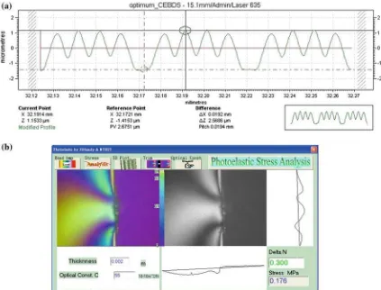
The 95 % confidence interval of S/N ratio for V-cut depth, V-cut angle, and residual stress are 5.091822< µconfirmation
< 11.83575; −20.2842 < µconfirmation < −15.5014;and 11.93522 < µconfirmation < 14.05634, respectively. The surface profile of V-cut microstructures and the residual stress under the optimal combination is shown in Fig.7. The S/N ratio (dB) derived from four verification data for the V-cut depth, V-cut angle, and residual stress are 10.91939, −14.4397, and 14.9668, respectively. Compared to trial no. 16 in L18 orthogonal array, which shows the best S/N ratio among all trials, the result of CEBDS is able to improve the
quality of V-cut angle and residual stress. However, the V-cut depth quality was deteriorated with the decrease of−4.38 dB. The 95 % Confidence Interval of experimental V-cut depth value is calculated as:
C I2=
Fα;1,v2×Verr or×
1
ne f f
+1
r
=
4.84x6.04048×
7 18+
1 4
=4.321978d B (8)
The 95 % confidence interval of S/N ratio for V-cut depth, V-cut angle, and residual stress are 6.597413< µconfirmation
< 15.24137; −17.7361 < µconfirmation < −11.1434; and 13.6897 < µconfirmation < 16.2438, respectively. The dia-gram for the CI of the V-cut depth, angle, and residual stress verification experiment values and theoretical predicted val-ues are shown in Fig.8. From the diagrams, the CI from the verification experiment and the theoretical predictions did indeed coincide; therefore the results from the experiment using CEBDS approach are indeed reliable had been proven.
Verification of reciprocal comparisons approach
Using Eq.6, the S/N ratio of optimal processing parameters for V-cut depth is 11.41823 dB. Confidence Interval (CI) of theoretically-predicted value is calculated using Eq.7,
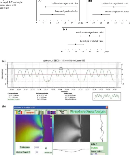
yield-ing 3.60468 dB. The 95 % confidence interval of S/N ratio for V-cut depth, V-cut angle, and residual stress are 7.81355 < µconfirmation < 15.02291; −20.2842 < µconfirmation < −15.5014;and12.57461 < µconfirmation < 14.79927, respectively. The surface profile of V-cut microstructures and
Fig. 8 Diagram for the CI of theaV-cut depthbV-cut angle andcresidual stress with CEBDS approach
theoretical predicted value confirmation experiment value confirmation experiment value
(
a
)
(b)
(c)
theoretical predicted value confirmation experiment value theoretical predicted value
F i g . 1 0 Diagram for the CI of theaV-cut depthbV-cut angle andcresidual stress, with reciprocal comparisons approach
(a) (b)
(c)
residual stress under the optimal combination is shown in Fig.9. The S/N ratio (dB) derived from four verification data for the V-cut depth, V-cut angle, and residual stress are 14.6251,−13.174, and 15.5299, respectively. Compared to trial no. 16 in L18 orthogonal array, which shows the best S/N ratio among all trials, the result of reciprocal compar-isons is able to improve the quality of V-cut angle and residual stress. The V-cut quality is a bit worse with the decrease of −0.674 dB. However, the total improvement for all qualities is +5.276 dB with more balanced manner without sacrific-ing one of the qualities. Obviously, the total improvements of all qualities in reciprocal comparisons obviously outper-form that in CEBDS method. The 95 % Confidence Inter-val of experimental V-cut depth Inter-value is calculated using Eq.8, yielding 4.505978 dB. The 95 % confidence interval of S/N ratio for V-cut depth, V-cut angle, and residual stress are 10.11911 < µconfirmation < 19.13107; −16.4701 <
µconfirmation <−9.87743; and 14.20946 < µconfirmation < 16.85025, respectively. The diagram for the CI of the V-cut depth, angle, and residual stress verification experiment val-ues and theoretical predicted valval-ues are shown in Fig.10. From the diagrams, the CI from the verification experiment and the theoretical predictions did indeed coincide; there-fore the results from the experiment using reciprocal com-parisons approach are indeed reliable had been proven. It can easily be observed that using the reciprocal comparisons approach to measure DMU’s efficiency in the proposed pro-cedure results in better outcome than the CEBDS approach (Abbas 2009). Thus, reciprocal comparisons are promising to be used in optimization problems for its simplicity and powerfulness.
Conclusion
The reciprocal comparisons approaches in DEA were pro-posed to find out the optimal processing parameters of injec-tion molding machine. The optimal processing parameters in reciprocal comparisons approach are A2,B3,C1,D3,E2,F3,
G1,H3, that is: the cooling time of 30 s, mold tempera-ture of 85◦C, melt temperature of 250◦C, injection speed of 195 mm/s, injection pressure of 240 MPa, packing pres-sure of 110 MPa, packing switching of 5 mm, and the pack-ing time of 3 s. The reciprocal comparisons methods were able to search optimal parameters combinations beyond the orthogonal array experimentation set. Confirmation exper-iments showed that the optimal parameters combination demonstrated qualities improvements in a more balanced manner. Compared with CEBDS approach, the reciprocal comparisons approach shows a better effectiveness because not only provides larger anticipated improvements in the responses, but also requires less computations since within-comparisons is not required. The reliability and repro-ducibility of the results were verified using 95 % confidence interval.
Acknowledgments This research was financially supported by the National Science Council of the Republic of China under Grant No. NSC 97-2622-E-011-001-CC3.
Appendix
Table 8 The efficiencies for all DMUs DMUj Factor
A B C D
Ej,1 Ej,2 Ej,1 Ej,2 Ej,3 Ej,1 Ej,2 Ej,3 Ej,1 Ej,2 Ej,3
DMU1 0.645 0.45 1 0.693 0.45 0.45 0.474 1.235 0.476 0.645 0.45
DMU2 0.786 0.742 0.956 0.766 0.742 0.742 0.766 0.954 0.786 0.786 0.742
DMU3 0.859 0.811 1 0.849 0.811 0.811 0.838 1 0.859 0.859 0.811
DMU4 0.824 0.778 1.04 0.825 0.778 0.778 0.804 0.985 0.824 0.824 0.778
DMU5 1 0.726 2.164 1 0.726 0.726 0.844 2.673 0.844 1 0.726
DMU6 0.715 0.611 1.127 0.803 0.611 0.611 0.637 1 0.647 0.715 0.611
DMU7 1 0.945 1.872 1.181 0.945 0.945 1.016 1.309 1.078 1 0.945
DMU8 0.136 0.09 0.205 0.137 0.09 0.09 0.135 0.153 0.146 0.136 0.09
DMU9 0.885 0.723 1.595 1.016 0.723 0.723 0.896 1 0.955 0.885 0.723
DMU10 0.428 0.288 0.858 0.437 0.288 0.288 0.334 1.059 0.334 0.428 0.288
DMU11 0.385 0.362 0.575 0.443 0.362 0.362 0.376 0.506 0.383 0.385 0.362
DMU12 0.808 0.763 1 0.787 0.763 0.763 0.787 1 0.808 0.808 0.763
DMU13 0.53 0.5 0.652 0.541 0.5 0.5 0.517 0.632 0.53 0.53 0.5
DMU14 1.026 0.969 1.487 1 0.969 0.969 1 1.291 1.086 1.026 0.969
DMU15 0.591 0.558 0.74 0.594 0.558 0.558 0.577 0.702 0.591 0.591 0.558
DMU16 2.02 1 3.745 2.218 1 1 1.585 3.683 1.624 2.02 1
DMU17 1.493 0.945 2.719 1.573 0.945 0.945 1 3.168 1 1.493 0.945
DMU18 0.217 0.158 0.47 0.217 0.158 0.158 0.183 0.58 0.183 0.217 0.158
DMUj Factor
E F G H
Ej,1 Ej,2 Ej,3 Ej,1 Ej,2 Ej,3 Ej,1 Ej,2 Ej,3 Ej,1 Ej,2 Ej,3
DMU1 1 0.45 0.476 0.476 1.236 0.45 0.45 0.476 2.398 0.878 0.45 0.474
DMU2 0.766 0.742 0.786 0.786 0.766 0.742 0.742 0.786 1.1 1.479 0.742 0.766
DMU3 0.839 0.811 0.859 0.859 0.859 0.811 0.811 0.859 1 1.454 0.811 0.838
DMU4 0.806 0.778 0.824 0.824 0.845 0.778 0.778 0.824 1 1.432 0.778 0.804
DMU5 2.164 0.726 0.844 0.844 2.577 0.726 0.726 0.844 4.979 1 0.726 0.844
DMU6 0.857 0.611 0.647 0.647 1.093 0.611 0.611 0.647 2.126 1.177 0.611 0.637
DMU7 1 0.945 1.078 1.078 1.311 0.945 0.945 1 2.744 2.251 0.945 1
DMU8 0.135 0.09 0.146 0.146 0.137 0.09 0.09 0.136 0.24 0.305 0.09 0.135
DMU9 0.884 0.723 0.955 0.955 1 0.723 0.723 0.885 2.193 1.993 0.723 0.884
DMU10 0.858 0.288 0.334 0.334 1 0.288 0.288 0.334 1.959 0.469 0.288 0.334
DMU11 0.39 0.362 0.383 0.383 0.51 0.362 0.362 0.383 0.965 0.668 0.362 0.376
DMU12 0.787 0.763 0.808 0.808 0.787 0.763 0.763 0.808 1.298 1.652 0.763 0.787
DMU13 0.52 0.5 0.53 0.53 0.563 0.5 0.5 0.53 0.731 0.899 0.5 0.517
DMU14 1 0.969 1.086 1.086 1 0.969 0.969 1.026 1.782 2.267 0.969 1
DMU15 0.578 0.558 0.591 0.591 0.61 0.558 0.558 0.591 0.738 1 0.558 0.577
DMU16 3.063 1 1.624 1.624 3.774 1 1 1.575 7.605 3.391 1 1.575
DMU17 2.581 0.945 1 1 3.154 0.945 0.945 1 6.235 2.088 0.945 1
R e f e r e n c e s
Abbas, A. R. (2009). Optimizing SMT performance using comparisons of efficiency between different systems technique in DEA.IEEE
Transactions on Electronics Packaging Manufacturing,32(4), 256–
264.
Abbas, A. R., & Mohammad, D. A. (2011). Solving the multi-response problem in Taguchi method by benevolent formulation in DEA.
Jour-nal of Intelligent Manufacturing,22(4), 505–521.
Anthony, J. (2000). Multi-response optimization in industrial experi-ments using Taguchi’s quality loss function and principal component analysis.Quality and Reliability Engineering International,16(1), 3–8.
Bociaga, E., Jaruga, T., Lubczynska, K., & Gnatowski, A. (2010). Warpage of injection moulded parts as the result of mould temper-ature difference.Archives of Materials Science and Engineering,
44(1), 28–34.
Choi, D. S., & Im, Y. T. (1999). Prediction of shrinkage and warpage in consideration of residual stress in integrated simulation of injection molding.Composite Structures,47(1–4), 655–665.
Cicek, A., Kivak, T., & Ekici, E. (2013). Optimization of drilling parameters using Taguchi technique and response surface method-ology (RSM) in drilling of AISI 304 steel with cryogenically treated HSS drills. Journal of Intelligent Manufacturing. doi:10. 1007/s10845-013-0783-5.
Cooper, W. W., Seiford, L. M., & Tone, K. (2006).Introduction to data
envelopment analysis and its uses. New York: Springer.
Dragan, K., Tomaz, K., Janez, M. K., Rajko, S., & Janez, G. (2013). The impact of process parameters on test specimen deviations and their correlation with AE signals captured during the injection moulding cycle.Polymer Testing,32(3), 583–593.
Faisal, A. A., Mahmoud, B., & Ibrahim, M. (2013). A combined ana-lytical hierarchical process (AHP) and Taguchi experimental design (TED) for plastic injection molding process settings.The
Interna-tional Journal of Advanced Manufacturing Technology, 66(5–8),
679–694.
Guilong, W., Guoqun, Z., & Xiaoxin, W. (2013). Effects of cavity sur-face temperature on mechanical properties of specimens with and without a weld line in rapid heat cycle molding. Materials and
Design,46, 457–472.
Hasan, O., Tuncay, E., & Ibrahim, U. (2007). Application of Taguchi optimization technique in determining plastic injection moulding process parameters for a thin-shell part.Materials and Design,28(4), 1271–1278.
Huang, M. S., Yu, J. C., & Lin, Y. Z. (2009). Experimental rapid surface heating by induction for micro-injection molding of light-guided plates.Journal of Applied Polymer Science,113(2), 1345–1354. Humberstone, M., Wood, B., Henkel, J., & Hines, J. W. (2012).
Dif-ferentiating between expanded and fault conditions using principal component analysis.Journal of Intelligent Manufacturing,23(2), 179–188.
Jui, W. P., & Ya, W. H. (2012). Light-guide plate using periodical and single-sized microstructures to create a uniform backlight system.
Optics Letters,37(17), 3726–3728.
Kazmer, D. O. (2007).Injection mold design engineering. Munich: Hanser Publishers.
Kuo, C. F. J., Su, T. L., Jhang, P. R., Huang, C. Y., & Chiu, C. H. (2011). Using the Taguchi method and grey relational analysis to optimize the flat-plate collector process with multiple quality characteristics in solar energy collector manufacturing.Energy,36(5), 3554–3562.
Kuo, C. F. J., Tu, H. M., Liang, S. W., & Tsai, W. L. (2010). Optimiza-tion of microcrystalline silicon thin film solar cell isolaOptimiza-tion process-ing parameters usprocess-ing ultraviolet laser.Optics and Laser Technology,
42(6), 945–955.
Lin, H. L. (2012). The use of the Taguchi method with grey relational analysis and a neural network to optimize a novel GMA welding process.Journal of Intelligent Manufacturing,23(5), 1671–1680. Muhammad, N., Manurung, Y. H. P., Jaafar, R., Abas, S. K., Tham, G.,
& Haruman, E. (2012). Model development for quality features of resistance spot welding using multi-objective Taguchi method and response surface methodology.Journal of Intelligent Manufacturing. doi:10.1007/s10845-012-0648-3.
Murakami, O., Kotaki, M., & Hamada, H. (2008). Effect of molecular weight and molding conditions on the replication of injection mold-ing with micro-scale V-groove features.Polymer Engineering and
Science,48(4), 697–704.
Nik, M. M., & Shahrul, K. (2011). Optimization of mechanical proper-ties of recycled plastic products via optimal processing parameters using the Taguchi method.Journal of Materials Processing Technol-ogy,211(12), 1989–1994.
Nor, H. M. N., Norhamidi, M., Sufizar, A., Mohd, H. I. B., Mohd, R. H., & Khairur, R. J. (2010). Parameter optimization of injection molding Ti-6Al-4V powder and palm stearin binder system for highest green density using Taguchi method. Key Engineering Materials, 443, 69–74.
Ross, P. J. (1996).Taguchi techniques for quality engineering(2nd ed.). New York: McGraw-Hill.
Sanchez, R., Aisa, J., Martinez, A., & Mercado, D. (2012). On the rela-tionship between cooling setup and warpage in injection molding.
Measurement,45(5), 1051–1056.
Saurav, D., Goutam, N., Asish, B., & Pradip, K. P. (2009). Application of PCA-based hybrid Taguchi method for correlated multicriteria optimization of submerged arc weld: a case study.The International
Journal of Advanced Manufacturing Technology,45(3–4), 276–286.
Shye, Y. H., Norhamidi, M., Abu, B. S., Abdolali, F., & Sriyulis, M. A. (2013). Effect of sintering temperature on the mechanical and physical properties of WC-10%Co through micro-powder injection molding(µPIM).Ceramics International,39(4), 4457–4464. Thian, E. S., Loh, N. H., Khor, K. A., & Tor, S. B. (2002).
Microstruc-tures and mechanical properties of powder injection molded Ti-6Al-4V/HA powder.Biomaterials,23(14), 2927–2938.
Umbrello, D., Ambrogio, G., Filice, L., Guerriero, F., & Guido, R. (2010). A clustering approach for determining the optimal process parameters in cutting.Journal of Intelligent Manufacturing,21(6), 787–795.
Yang, Y. S., Shih, C. Y., & Fung, R. F. (2012). Multi-objective optimiza-tion of the light guide rod by using the combined Taguchi method and Grey relational approach.Journal of Intelligent Manufacturing. doi:10.1007/s10845-012-0678-x.