COMPARISONS BETWEEN DIFFERENT INTERPOLATION TECHNIQUES
G. Garnero a, *, D. Godoneb a
DIST, Università e Politecnico di Torino - Torino, Italy - [email protected] b
DISAFA, Università di Torino - Torino, Italy - [email protected]
KEY WORDS: DTM, Accuracy, IntesaGIS, LIDAR, Modelling, Specifications, Validation.
ABSTRACT
Digital terrain models are key tools in land analysis and management as they are directly employable in GIS systems and other specific applications like hydraulic modelling, geotechnical analyses, road planning, telecommunication, and many others. TIN generation, from different kind of measurement techniques, is ruled by specific regulations. Interpolation techniques to compute a regular grid from a TIN, are, instead, still lacking in specific regulations: a unitary and shared methodology has not already been made compulsory in order to be used in cartographic production while generating digital models. Such ambiguity obviously involves non univocal results and can affect precision, which can lead to divergent analyses on the same territory.
In the present study different algorithms will be analysed in order to spot an optimal interpolation methodology. The availability of the recent digital model produced by the Regione Piemonte with airborne LIDAR and the presence of sections of testing realized with higher resolutions and the presence of independent digital models on the same territory allow to set a series of analysis with consequent determination of the best methodologies of interpolation.
The analysis of the residuals on the test sites allows to calculate the descriptive statistics of the computed values: all the algorithms have furnished interesting results; all the more interesting, notably for dense models, the IDW (Inverse Distance Weighing) algorithm results to give best results in this study case. Moreover, a comparative analysis was carried out by interpolating data at different input point density, with the purpose of highlighting thresholds in input density that may influence the quality reduction of the final output in the interpolation phase.
* Corresponding author.
1. INTRODUCTION 1.1 DTM
Digital Terrain Models (DTM) are a resource in environment and land-related applications. They can be employed in several ways in order to have a thorough understanding of a given investigated area by extracting morphometric parameters (Pirotti and Tarolli, 2010) or to perform complex analyses on the standalone DTM (Guarnieri et al., 2009) or by combining it with other data sources with modelling purposes (Barbarella and Fiani, 2012, Barbarella and Fiani, 2013, Godone et al., 2011).
Airborne LIDAR (Wehr and Lohr, 1999) is a powerful tool to survey high-resolution and high-accuracy DTM in large areas (Guo et al., 2010; Pirotti et al., 2013). The output of a LIDAR survey is a point cloud that needs to be interpolated in order to provide a continuous surface to the final user (Kraus and Pfeifer, 2001). The choice of the interpolator and the cell size plays an important role in the quality of the output DTM (Bater and Coops, 2009).
1.1 IntesaGISDB’s features
The official working group called "IntesaGIS", has tried to establish a legal framework in the sphere of Italian cartography since 1996, and a series of documents has been developed to define some specific references on digital models. In summary:
the change in trend is represented by the fact that the main product is now represented by the DTM, while contour lines assume only a function of cartographic representation, derived from the same digital model and
aimed to improve map readability, while, processing favours the use of the DTM;
the specification defines a set of quality requirements, which the DTM must meet, from the accuracy point of view, in particular by establishing a series of different Levels, each one characterized by the accuracy and resolution of the output grid;
specifications for the production of digital models are also defined, including:
o the production of a TIN is ordinarily expected as a source of the regular grid for the DTM interpolation; o for the production of DTMs it is necessary to employ
all available information related to the ground (roads, built, hydrography, etc, restricted to those elements whose coordinate is referred to the ground);
o for the generation of the digital model it is necessary to integrate with mass points and breaklines uniquely surveyed with the aim of DTM production, without cartographic valence. The measurement of these points should be carried out by the use of digital photogrammetry, involving autocorrelation techniques, or LIDAR, in accordance of the accuracy Level desired.
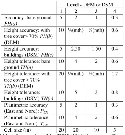
In any case, while the TIN production is ruled (Table 1), nothing is specified concerning cloud point interpolation for DTM computation purposes.
Level - DEM or DSM
Table 1. Last version of the CISIS (2011) document –―Large scale orthoimagery and elevation models – Guidelines" shows
Level values: mth = mean tree height
The table is not complete: higher level DEMs are missing.
2. MATERIALS AND METHODS 2.1 Interpolation techniques
Interpolation tools available in geographical information systems are useful and allow the operator to easily perform different kind of elaborations and to display them graphically in order to show the results in a way intelligible also to non-skilled subjects.
Interpolators are divided in two typologies (Hartkamp et al., 1999):
1. deterministic; 2. stochastic.
These interpolators use a linear combination of known functions with different weighting and neighbouring search schemes: data that are closer to interpolation point have more influence (weight), during the computations, in comparison with faraway ones, according to the First Law of Geography (Tobler, 1970). Interpolators could be defined as weighted average methods, with similar processing concept; the operator, in fact, needs to compute an unknown value, at an unsampled location, given a set of neighbouring sampled values, collected at locations neighbouring the unknown one; the quantity of neighbouring points included in the search radius directly affects the final surface smoothing and the computing time.
The interpolation procedure consists in the definition of the search area or neighbourhood around the unknown point, the detection of the observed data points within the previously defined neighbourhood and, finally, the assignment of appropriate weights to each of the observed data points. The interpolation methods differ in the weighing of computing samples (Wong et al., 2004).
Interpolation and values sampling have been carried out in ESRI ArcGis rel. 10.1 (Booth, 2000; McCoy and Johnston, 2002) by the employment of Python scripting (van Rossum and Drake, 2001). Residuals and statistical analyses have been executed in R environment (R Development Core Team, 2010).
In the following paragraph, the interpolators employed in the work are briefly described.
2.1.1 IDW
The Inverse Distance Weighing (IDW) interpolator is an automatic and relatively easy technique, as it requires very few parameters from the operator, such as search neighbourhood parameters, exponent and eventually smoothing factor, from the operator (Hessl et al., 2007). It is particularly suitable for narrow datasets, where other fitting techniques may be affected by errors (Tomeczak, 2003). The process is highly flexible and allows estimating dataset with trend or anisotropy, in search neighbourhood shaping. Anyhow interpolator’s output may be
affected by ―bull’s eyes‖ or terraces (Burrough and McDonnel,
1988; Liu, 1999).
IDW directly implements the assumption that a value of an attribute at an unsampled location is a weighted average of known data points within a local neighbourhood surrounding the unsampled one (Mitas and Mitasova, 1999), as the The separation distancehij between a known and unknown point is measured with is euclidean distance:
2 2y
x
h
ij
(2)where x and y are the distances between the unknown point j
and the sampled one i according to reference axes.
2.1.2 Spline
Splines (Johnston et al., 2001) are interpolators that fit a function to sampled points. The algorithm uses a linear combination of n functions, one for each known point.
1Weights are assigned according to the distance of known points, under the constraint that, in their locations, the function must give the measured value. This conditions lead to the computation of a system of N equations with N unknowns with a unique solution.
Splines include different kinds of functions:
Thin-plate Spline function:
Completely regularized Spline function:
E
Spline with tension function:
E
r = distance between the point and the sample
σ = tension parameter
E1 = exponential integral function
Ce = constant of Eulero (0,577215)
K0= modified Bessel function.
Splines functions are slightly different, each one has a different smoothing parameter depending on the σ parameter. In every method, the higher the value of σ, the higher the gradualness of
the variation, except for the ―Inverse multi-quadric‖ where the
opposite condition is true.
In the following analyses only two Splines were available, according to the selected GIS package ArcGIS by ESRI): the Regularized and the Tension one. The Regularized Spline creates a smooth, gradually changing surface.
The regularizing parameter is in fact employed to achieve a smoother solution: e.g. a small value results in a close approximation of the data, while a large one results in a smoother solution (Gousie and Franklin, 2005).
The Tension Spline creates a less smooth surface with values more constrained by the sample data range: changing the value of the tension parameter tunes the surface from a stiff plate into an elastic sheet (Mitas et al., 1997).
2.1.3 Natural neighbours
Natural neighbour (NN) interpolation finds the closest subset of input points to an unknown point, and applies weights to them based on proportionate areas in order to interpolate a value (Sibson, 1981). The natural neighbours of any point are those associated with the neighbouring Voronoi polygons. Initially, a Voronoi diagram is constructed from all given points and a new Voronoi polygon is then created around the interpolation point. The proportion of overlap between this new polygon and the initial polygons are then used as weights.
Natural Neighbours is local, using only one subset of points that surround the unknown point. It infers no trends and will produce no peaks, pits, ridges or valleys not already represented by the input data.
The surface passes through the input samples and it is smoothed everywhere except at the locations of the input samples. It adapts locally to the structure of the input data, requiring no input from the user pertaining to search radius, sample count, or shape. It works equally well with regularly and irregularly distributed data (Watson, 1992).
2.2 LIDAR survey
Data for the present work have been provided by Regione Piemonte survey aimed to the production of a digital orthoimage at 1:5000 scale and a digital terrain model at Level4 in accordance with Intesa specifications (CISIS, 2011). LIDAR survey has been carried out by the employment of ALS 50 II sensor (Leica Geosystems) with MPIA (Multiple Pulse In Air) technology with the following features (Dold and Flint, 2007):
- Maximum Pulse Rate: 150000 Hz (150.000 points/second);
- Maximum scanning frequency: 90 Hz (90 lines/second); 4 echoes (1º, 2º, 3ºand last);
- Flying height: 200 - 6000 mabove ground; - Field Of View (FOV): 10º – 75 º; - Side overlap: 200 - 600 m; - Intensity measured each echo.
In addition to the ordinary survey, in a portion of Regione Piemonte, a more detailed one has been required. It has been characterized by the following parameters:
- FOV (Field Of View): 58º; - LPR (Laser Pulse Rate): 66.400 Hz; - Scan Rate: 21.4 Hz;
-Average Point Density:0.22 pts/m²; -Average Point Spacing: 2.12 m;
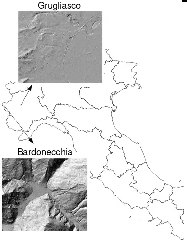
2.3 Datasets
The described algorithms have been applied to two datasets (Figure 1), characterized by different morphological features. The first one, Bardonecchia (45° 4′ N; 6° 42′ E), is located in a
Figure 1. Study sites
2.3.1 Bardonecchia
The dataset has been surveyed during the measurement campaign mentioned above and filtered in order to extract only ground points, the amount of input data is 12017944 with a density of 1 point every 3.26 m². The survey encompasses approximately 39.20 Km².
From this huge amount of data, a test subset, consisting of the 1% of the total, has been extracted in order to perform validation (Bater and Coops, 2009).
The rest of the points have been iteratively subsampled, using
SubsetFeatures ArcMap command, with the aim of computing
different input subsets to be employed in the interpolation
Table 2. Bardonecchia test site, input subsets
2.3.2 Grugliasco
An analogous procedure has been carried out in the Grugliasco site. The initial survey covers an area of 38.44 Km² and 10965358 ground points were extracted with a density of 1 poin every 3.54 m². The following table (
Table 3) reports the features of the input subsets.
Name
Table 3. Grugliasco test site, input subsets
2.4 DTM analysis
Every input subset has been interpolated in ESRI ArcMap by different algorithms with default input parameters (Mitas and Mitasova, 1999) i.e. IDW (Power = 2, Search radius = variable, Maximum number of points = 12), Natural Neighbours (No parameters), Splines (Weight = 0.1, Maximum number of points = 12). Moreover splines have been employed in three different ways by selecting Regularised, Tension and Tension with Barriers. Barriers have been obtained by breaklines, in three dimensional shape file format, provided with the input datasets.Kriging has been excluded as its use without the exploitation of its data exploratory capabilities makes it mathematically similar to splines (Cressie, 1991).
Each subset has been interpolated at 5x5, 10x10 and 20x20 metres cell size, by every listed method. Resulting grids have been sampled using the designated methods and extracted
elevation values have been subtracted from test points’
elevation in order to obtain residuals and compute descriptive
statistics with the aim of pointing out the best algorithm’s
performance.
3. RESULTS AND DISCUSSION 3.1 Quality assessment
Only the IDW and Natural neighbours methods have been able to generate the entire set of grids; splines have encountered difficulties in the interpolation of denser dataset thus grids from Base0 to Base10 have not been computed, perhaps due to the overrun of the memory allocated to the processing.
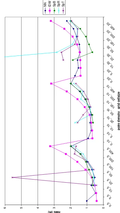
The residual computed on the test subsets have allowed to compute descriptive statistics for each interpolator at every resolution. Figure 2 and figure 3show the comparison of RMS for the two sites. The reported analysis are assumed to be independent from the LIDAR survey accuracy, and therefore only the computed residuals are related to the different point density and of algorithm choice.
Bardone
Figure 2. Bardonecchia site, quality assessment (NN = Natural Neighbors, IDW = Inverse Distance Weighing, SpB = Tension Spline with Barriers, SpR = Regularized Spline, SpT = Tension
Spline)
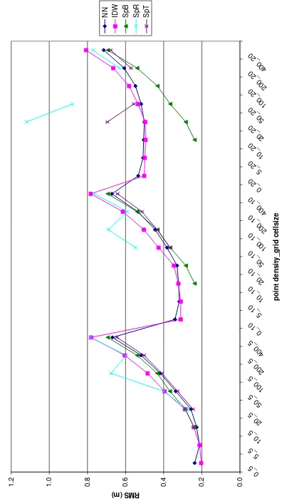
Grugli
Figure 3. Grugliasco site, quality assessment (NN = Natural Neighbors, IDW = Inverse Distance Weighing, SpB = Tension Spline with Barriers, SpR = Regularized Spline, SpT = Tension
Spline)
Some interpolation methods (in particular splines) with certain input resolutions have produced unexpected results with peaks in residual values.
RMS values, resulting from the different available subsets, grow, as it was logical to assume, with decreasing density of input points available in accordance with the findings of Anderson et al (2006).
RMS also undergoes a growth trend as a function of grid spacing product, with a trend relatively more significant in areas characterized by simpler morphology (Godone and Garnero, 2013).
When input points density decreases, the algorithm IDW looks less performing than others, which do have a more homogeneous behaviour.
4. CONCLUSIONS
In DTM production the testing procedures ordinarily include the acquisition of GPS transects or the survey of grids characterized by precision and densityhigher than the one to be validated.According to these methods the procedure implemented in the present work seems meaningful to represent the testing procedures.
Findings obtained from the analysesmay be helpful to define, in the case histories and with interpolation algorithms
considered,the minimum density of points required to obtain the precision expected by the various Levels.
Specifically, concerning land with complex morphology (Bardonecchia) the remarks are as follows:
in the case of the restrictive Level 4, which is associated with a grid spacing of 5 m, only the most extreme density, with one point every 3/5 square meters, can guarantee the satisfaction of the required accuracies;
concerning Level 3, which is associated with a grid spacing of 10 m, it is not possible to descend to lower densities at one point every 20 square meters as, in addition to the contributions in terms of RMS data by methods of interpolation, it is still necessary to evaluate the contributions of the measurement methods, not considered the effects of this work;
Levels 2 and 1, which are associated with a grid spacing of 20 m.According to the accuracies of the LIDAR measures currently reached, it is not advisable to decrease the resolution under one point every 100 square meters in the case of Level 2, while for Level 1 also the lowest resolution considered is sufficient.
In the case of the situation of the City of Grugliasco, in absolute terms the values are much lower, as it is natural to expect. From the analysis of the graph shown in Figure 3, a quite similar behaviour in relative terms is remarked :
in the case of the Level 4, only the density of more than one point every 20 square meters can guarantee the satisfaction of the required accuracies;
for the others Levels, all densities taken into consideration can be usefully used.
5. ACKNOWLEDGEMENTS
LIDAR data have been provided by Gianni Siletto, Regione Piemonte - Direzione Programmazione Strategica, Politiche territoriali ed Edilizia. Settore Infrastruttura geografica, strumenti e tecnologie per il governo del territorio.
6. REFERENCES
Ajmar, A., Boccardo, P., Tonolo, F. G., 2011. Earthquake damage assessment based on remote sensing data. The Haiti case study. Italian Journal of Remote Sensing / RivistaItaliana Di Telerilevamento, 43(2), 123-128
Anderson E. S., Thompson J. A., Crouse D. A., Austin R. E., 2006. Horizontal resolution and data density effects on remotely sensed LIDAR-based DEM, Geoderma, 132(3–4), pp. 406 – 415
Barbarella, M., Fiani, M., 2013. Monitoring of large landslides by Terrestrial Laser Scanning techniques: field data collection and processing., European Journal Of Remote Sensing, vol. 46, year: 2013 Pages: 126 - 151 DOI: 10.5721/EuJRS20134608
Barbarella M., Fiani M., 2012. Landslide monitoring using terrestrial laser scanner: georeferencing and canopy filtering issues in a case study, ISPRS International Archives of the Photogrammetry, Remote Sensing and Spatial Information Sciences. vol. XXXIX-B5, p. 157-162
Bater, C.W., Coops, N.C., 2009. Evaluating error associated with lidar-derived DEM interpolation, Computers &
Geosciences, 35, 2, 289-300.
Booth, B., 2000. Using ArcGIS 3D Analyst. Environmental Systems Research Institute.
Burrough, PA., McDonnell, R.A., 1988. Principles of
Geographical Information Systems. Oxford University Press,
Oxford, 1988.
CISIS (Centro Interregionale di Coordinamento e Documentazione per le Informazioni Territoriali), 2011.
Ortoimmagini e modelli altimetrici a grande scala - Linee
Guida, available at http://www.centrointerregionale-gis.it
Cressie, N. A. C., 1991. Statistics for spatial data. John Wiley, New York, 920 pp.
Dold, J., Flint, D., 2007. Leica Geosystems photogrammetric
sensor and workflow developments in Fritsch D. (ed.)
Photogrammetric Week 2007, Stuttgart, Deutschland, pp. 3 - 14
Godone, D., Garnero, G., 2013. The role of morphometric parameters in Digital Terrain Models interpolation accuracy: a case study, European Journal of Remote Sensing, 46, pp. 198-214
Godone, D., Garnero, G., Filippa, G., Freppaz, M., Terzago, S., Rivella, E., Salandin, A., Barbero, S., 2011. Snow cover extent and duration in MODIS time series: A comparison with in-situ measurements (ProvinciaVerbanoCusioOssola, NW Italy), International Conference on Multimedia Technology, Hangzhou, China, pp. 4092-4095
Gousie, M.B., Franklin, W.R., 2005. Augmenting grid-based contours to improve thin plate dem generation.
Photogrammetric Engineering & Remote Sensing, 71, 69-79.
Guarnieri, A., Vettore, A., Pirotti, F., Menenti, M., Marani, M., 2009. Retrieval of small-relief marsh morphology from Terrestrial Laser Scanner, optimal spatial filtering, and laser return intensity, Geomorphology, Volume 113, Issues 1–2, 1, 12-20
Guo, Q., Li, W., Yu H., Alvarez, O., 2010. Effects of topographic variability and lidar sampling density on several DEM interpolation methods, Photogrammetric Engineering &
Remote Sensing, 76(6), pp. 701 – 712
Hartkamp, A.D., K. De Beurs, A., Stein, J.W., White., 1999. Interpolation Techniques for Climate Variables. NRG-GIS Series 99-01. Mexico, D.F.: CIMMYT.
Hessl, A., Miller, J., Kernan, J., Keenum, D., McKenzie, D., 2007. Mapping Paleo-Fire Boundaries from Binary Point Data: Comparing Interpolation Methods, The Professional
Geographer, 59 (1), pp. 87-104
Johnston, K., VerHoef, J., Krivoruchko, K., Neil, L., 2001.
Using ArcGIS™ Geostatistical Analyst, ESRI™, USA
Kraus, K, Pfeifer, N., 2001. Advanced DTM generation from LIDAR data, International Archives of the Photogrammetry,
Remote Sensing and Spatial Information Sciences, XXXIV (Pt.
3/W4), pp. 23–30.
Liu, H., 1999. Development of an Antarctic digital elevation model: Columbus, Ohio. The Ohio State University, Byrd Polar Research Center, BPRC Report No. 19, pp.157
McCoy, J., Johnston, K., 2002. Using Arcgis Spatial Analyst. Environmental Systems Research Institute.
Mitas, L., Mitasova, H., Brown, W.M., 1997. Role of dynamic cartography in simulations of landscape processes based on multi-variate fields,Computers & Geosciences, 23: 437–46
Mitas, L., Mitasova, H. 1999. Spatial Interpolation. In: Longley, P. Goodchild, M.F., Maguire, D. and Rhind, D. (eds.) Geographical Information Systems. 2nd Edition. Vol. 1: Principles and Technical Issues: 481-492.
Pirotti, F., Tarolli, P., 2010., Suitability of LiDAR point density and derived landform curvature maps for channel network extraction, Hydrological Processes, 24 (9), pp. 1187 – 1197.
Pirotti, F., Guarnieri, A., Vettore, A. 2013. State of the art of ground and aerial laser scanning technologies for high-resolution topography of the earth surface. European Journal of
Remote Sensing, 46:66-78. doi: 10.5721/EuJRS20134605
R Development Core Team 2010. ―R: A language and environment for statistical computing‖. R Foundation for Statistical Computing, Vienna, Austria.
Sibson, R., 1981. A Brief Description of Natural Neighbor
Interpolation, Chapter 2 in Interpolating multivariate data,
John Wiley & Sons, New York, 1981, pp. 21-36.
Tobler, W.R., 1970. A computer movie simulating urban growth in the Detroit region, Economic Geography, 46(2): 234-240.
Tomeczak, M., 2003. Spatial Interpolation and its Uncertainity using Automated Anisotropic Inverse Distance Weghing (IDW)
– Cross-validation/Jacknife Approach in Mapping radioactivity
in environment, in. Dubois G., Malczewski J., de Court M.,
(eds.) Spatial Interpolation Comparison, European Commission
– Joint Research Centre, 51-62
Van Rossum, G., Drake, F.L., 2001. Python Reference Manual, PythonLabs, Virginia, USA, Available at http://www.python.org
Watson, D., 1992. Contouring: A Guide to the Analysis and
Display of Spatial Data,Pergamon Press, London, 1992.
Wehr, A., Lohr, U., 1999. Airborne laser scanning—an introduction and overview, ISPRS Journal of Photogrammetry
and Remote Sensing, 54, 2–3, 68-82.
Wong, D.W., Yuan, L., Perlin, S.A., 2004. Comparison of spatial interpolation methods for the estimation of air quality data. Journal of Exposure Science and Environmental
Epidemiology, 14, 404-415.