CPT-based Interpretation of Pile Load Tests in Clay-Silt Soil
Prakoso, W.A.1)
Abstract: Two pile axial load tests were performed in a site in Depok, West Java. The soil of the site is predominantly a silt-clay soil, characterized by seven mechanical cone penetration tests (CPTs). The piles were 5.5 m long and 11.5 m long, 250 mm square piles. The results of the static load tests showed that the ultimate capacities were achieved. The axial load tests were subsequently back-analyzed using an axisymmetric finite element model using PLAXIS. In the back-analyses, the soil modulus and shear strength in the model, using the cone penetration resistance as the reference, were adjusted so that the numerical load-settlement curves matched the actual curves. The results of the back-analyses are then synthesized with the results of the CPTs, and are compared with available design guidelines. Some recommendations are then proposed.
Keywords: Cone penetration tests, driven piles, ultimate capacity, finite element analysis.
Introduction
In the design of axially loaded piles, the side resistance and tip resistance of piles are of great interest. Numerous laboratory and field pile load tests have been conducted to provide better estimates of these resistances, in which these resistances are subsequently correlated to some soil parameters obtained from laboratory and field soil tests [1]. The cone penetration test (CPT) is a type of soil tests widely used to predict the axial ultimate capacity of pile foundations [2,3]. The cone penetration resistance and sleeve friction data are used to predict the side resistance and tip resistance of piles using empirical equations. It is noted however that, in Indonesia, most of the empirical equations typically used were developed from abroad, and used without proper evaluation.
To evaluate these empirical equations, data of piles axially loaded to their ultimate capacities have to be collected and subsequently analyzed; this paper is a contribution to this evaluation process. During the construction of a six-story building in Depok, West Java, axial load tests were performed on two piles, in which the load-settlement curves from the load tests indicated that the ultimate capacities of both piles were reached. The 5.5 m long and 11.5 m long piles are 250 mm square concrete driven piles.
1 Civil Engineering Department, University of Indonesia, Depok 16424, INDONESIA
Email: [email protected]
Note: Discussion is expected before June, 1st 2011, and will be published in the “Civil Engineering Dimension” volume 13, number 2, September 2011.
Received 20 April 2010; revised 19 August 2010; accepted 9 September 2010.
These unique features (axial load tests of piles with different lengths and load-settlement curves indicating failures) provide insights into the behavior of pile foundation in this type of soil. The soil of the site is predominantly a silt-clay soil as characterized by seven mechanical CPTs.
To examine the observed pile foundation behavior, the axial load tests were subsequently back-analyzed using an axisymmetric finite element model. In the back-analyses, the soil parameters were adjusted so that the numerical load-settlement curves matched the actual curves. The cone penetration resistance was used as the reference in the back-analysis process.
This paper describes the geotechnical conditions and the axial load tests performed. It continues with a discussion on the back-analysis process. The results are then synthesized with the results of the CPTs, and are compared with available design guidelines. It concludes by highlighting the key observations.
Geotechnical Conditions
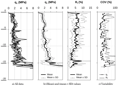
1b. In addition, the variability, represented by the coefficient of variation (COV = standard deviation/ mean), for both qc (square & line) and Rf (line) is shown in Figure 1c. Based on the CPT results, the ground can be simplified into the following four soil layers: (1) depth = 0–5.0 m, (2) depth = 5.0–11.0 m, (3) depth = 11.0–14 m, and (4) depth = 14.0–16.0 m.
The Robertson’s CPT interpretation procedure [5] was modified by the author to accommodate the use of mechanical CPTs in this study; the normalized cone resistance Q and the normalized friction ratio F respectively are given by the following:
Q = (qc – σv) / σ’v (1)
F = fs / (qc – σv) (2)
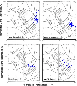
in which σv = overburden total vertical stress and σ’v = overburden effective vertical stress, and fs = sleeve friction. The Q and F profiles, along with the qc profiles, are shown as Figure 2; it is noted that the four soil layers identified above are confirmed using this approach. The Q and F values are subsequently plotted on the Robertson Q-F chart [4] shown as Figure 3. The first layer is predominantly in Zone 3 (silty clay to clay) with higher over-consolidation ratios (OCR), the second layer is predominantly in Zone 3 with lower OCR, and the third layer is predominantly in Zone 4 (clayey silt to silty clay)
with relatively low OCR. The fourth layer is a mixture of Zones 3 to 5 materials. Although it was based on electric CPT data, the Robertson Q-F chart provides reasonable results for the mechanical CPT data in comparison with deep boring data from the same site.
The qc is also corrected to the overburden effective vertical stress of 100 kPa. The overburden corrected cone penetration resistance, qc1, is computed by using an overburden correction factor CN as follows:
qc1 = CN⋅ qc (3)
In this paper, the CN expression proposed by Liao & Whitman [6] was used:
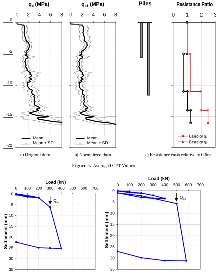
CN = (Pa / σ’v) 0.5≤ 1.7 (4) in which Pa = 100 kPa and σ’v = overburden effective stress in kPa. The qc1 mean values and the mean ± standard deviation values are shown in Figure 4, along with those of qc.
The difference in qc and qc1 values with depth is represented by the resistance ratio, in which the average qc and qc1 values in the first layer is used as the reference value. As shown in Figure 4c, qc tends to increase with depth, while qc1 tends to decrease and to increase with depth.
-15
-20 0
-5
-10
0 2 4 6 8
qc (MPa)
0 2 4 6 8
qc (MPa)
0 5 10 15
Rf (%)
0 100
COV (%)
Mean Mean ± SD
Mean Mean ± SD
qc Rf
a) All data b) (Mean) and (mean ± SD) values c) Variability
-20 0
-5
-10
-15
0 2 4 6 8
qc (MPa)
Mean Mean ± SD
1 10 100 1000 Q
0 5 10 15
F
Mean Mean ± SD
Mean Mean ± SD
Figure 2. Q and F Profiles
N
or
m
al
iz
ed C
one R
es
is
tanc
e,
Q
Layer (1): depth = 0 -5 m
Layer (2): depth = 5 - 11 m
N
o
rm
al
iz
ed
C
one
R
es
is
tanc
e
, Q
Layer(3): depth = 11 - 14 m
Layer(4): depth = 14 - 16 m
Normalized Friction Ratio, F (%)
Axial Load Tests
Two of the 250-mm-square-concrete piles were driven using a 15 kN drop hammer to depths of 5.5 m and 11.5 m, and the tip elevation of these piles relative to the CPT results are shown in Figure 4. Static axial load tests were subsequently conducted for the two piles in accordance with ASTM D1143 [7]. The load frame consisted of a kentledge system
and a hydraulic jack. The applied load was measured with a pressure gauge calibrated for the hydraulic jack. Pile settlement was measured with four dial gauges capable of reading movements of 0.01 mm. The piles were loaded in increments of 100 kN.
The results of the two pile load tests are shown in Figure 5. The 5.5 m long pile was loaded in two cycles, while the 11.5 m long pile was loaded in three
-20 0
-5
-10
-15
0 2 4 6 8
qc (MPa)
Mean Mean ± SD
0 2 4 6 8
qc1 (MPa)
Mean Mean ± SD
Piles
0 1 2 3
Resistance Ratio
Based on qc
Based on qc1
a) Original data b) Normalized data c) Resistance ratio relative to 0-5m
Figure 4. Averaged CPT Values
0
5
10
15
20
25
30
35
0 100 200 300 400 500 600 700 Load (kN)
Settl
e
m
ent (mm)
QL2
0
5
10
15
20
25
30
35
0 100 200 300 400 500 600 700
Load (kN)
S
e
ttlem
en
t (m
m
)
QL2
cycles. The axial load tests were terminated as the pile settlement became greater than 25 mm. Both load tests ended in less than 12 hours. The load-settlement curves of both piles indicate that the ultimate capacity of the piles have been achieved.
The L1-L2 method proposed by Hirany and Kulhawy [8] was used for interpreting the “failure” load or “ultimate” capacity of foundations. A typical foundation load-displacement curve has an initial elastic region, and the load defining the end of this region is interpreted as QL1. In the concluding part of the load-settlement curve, the load at the initiation of the final linear region is defined as QL2. The load level between QL1 and QL2 comprises the nonlinear transition region. The QL2 is defined as the “interpreted ultimate load”. Based on these load-displacement curves and the L1-L2 method, the QL2 of the 5.5 m long pile is 300 kN, while the QL2 of the 11.5 m long pile is 500 kN.
Curve-matching Numerical Analyses
The axial load tests were subsequently back-analyzed using PLAXIS [9]. In these curve-matching back-analyses, the soil modulus and shear strength in the model were adjusted so that the numerical load-settlement curves matched the actual curves.
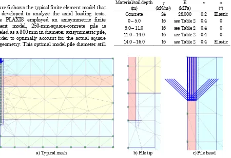
Figure 6 shows the typical finite element model that was developed to analyze the axial loading tests. Since PLAXIS employed an axisymmetric finite element model, 250-mm-square-concrete pile is modeled as a 300 mm in diameter axisymmetric pile, in order to optimally account for the actual square pile geometry.This optimal model pile diameter still
caused +13% error in the tip resistance area and -6% error in the side resistance area. The model used 15-node triangular elements for the pile and soil elements. The vertical side boundaries were horizontally restrained, while the horizontal bottom boundary was both horizontally and vertically restrained. A Mohr-Coulomb model with a soil friction angle, φ = 0 condition was used to describe the soil behavior; this model was chosen so that, for any given layer, the soil strength around the pile tip and the side resistance would not vary with depth. The soil layer with depth greater than 14 m and the pile concrete were modeled as a linear-elastic material. Zero-thickness, 10-node interface elements were used between the pile and the surrounding soil, including for the pile tip (Figure 6b); the interface elements had the same constitutive model as the soil elements. The soil parameters are given in Tables 1 and 2.
Displacement-controlled analyses were performed for the pile models. The displacement was applied to the pile head (Figure 6c), and the load was the output of the calculation procedure. The load-displacement curves were generated at the center point of the pile head.
Table 1. Model Properties
Material/soil depth γ E ν φ
(m) (kN/m3) (MPa) (°)
Concrete 24 28,000 0.2 Elastic
0 – 5.0 16 see Table 2 0.4 0
5.0 – 11.0 16 see Table 2 0.4 0
11.0 – 14.0 16 see Table 2 0.4 0
14.0 – 16.0 16 see Table 2 0.4 Elastic
a) Typical mesh b) Pile tip c) Pile head
Table 2. Soil Properties
Series I
Sub-series I-A Sub-series I-B Series II Depth (m) qc1 average values for depth = 0 – 5.0 m, respectively, based on resistance ratio shown in Figure 3c; Series I: based on qc resistance ratio; Series II: based on qc1 resistance ratio
Table 3. Comparison of Interpreted Pile Capacity Interpreted ultimate capacity (kN)
Series I Pile length
(m) Actual load
test Sub-series I-A
Sub-series I-B Series II
5.5 300.0 299.6
Two series of analyses were performed to match the interpreted ultimate loads and the initial part of the
load-settlement curve of each numerical model to that of the actual corresponding curve. In Series I, the soil elastic modulus and cohesion values were set based on the qc resistance ratio, while in Series II, the values were set based on the qc1 resistance ratio (Figure 4c). Series I consisted of two sub-series, in which the sub-series I-A was performed to match the load-settlement curve of the 5.5 m long pile, while the sub-series I-B was performed to match the curve of the 11.5 m long pile. Table 2 summarizes the soil properties used for all the series.
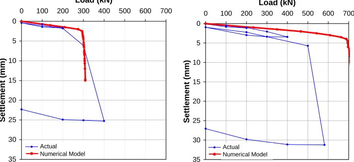
The load-settlement curves of all series are shown in Figures 7 and 8, compared with those of the actual load tests. For Series I, Figure 7a shows that, when the results for the 5.5 m long pile were matched, the results for the 11.5 m long pile could not be matched. On the other hand, Figure 7b shows that, when the results for the 11.5 m long pile were matched, the results for the 5.5 m long pile could not be matched. Table 3 summarizes the difference in the interpreted ultimate loads from both the load tests and the numerical analyses, which is about 30 – 40%.
0
a) Comparison for Sub-Series I-A Soil Properties
0
b) Comparison for Sub-Series I-B Soil Properties
0
Figure 8. Comparison of Results of Load Tests and Series II Numerical Analyses
0
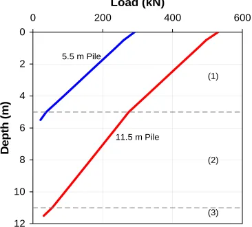
For Series II (resistance ratio based on qc1), Figure 8 shows that the load-settlement curves of both the 5.5 m long and 11.5 m long piles could be matched with the same soil properties. As indicated by Table 3, the difference in the interpreted ultimate loads is about 5%. The pile load distribution with depth at the interpreted ultimate load QL2 for both pile models is shown as Figure 9.
Discussion
The calculated side resistance of the piles is represented by the cohesion values in Table 2, and it ranges from 40 to 54 kPa. The calculated tip resistance of the piles was obtained from the normal stresses of the interface elements in the pile tip area of the pile models; the calculated tip resistance for the 5.5 m long pile is 308.8 kPa, while that for the 11.5 m long piles is 443.3 kPa. It is noted that the calculated tip resistance values are considered lower bound values, as the calculated load-settlement curves show flat plastic behavior, while the actual curves exhibit some strain hardening behavior.
Figure 9 indicates that the contribution of the pile tip to the overall ultimate capacity was relatively small. For the 5.5 m long pile, the calculated tip resistance is about 6% of the calculated pile ultimate capacity. For the 11.5 m long pile, the calculated tip resistance is about 4% of the calculated ultimate capacity. It can be concluded therefore that both piles behaved essentially as friction piles.
The 250-mm-square-concrete piles, according to the Canadian Foundation Engineering Manual (CFEM) [2], are within Group IIA. The CFEM sets that the maximum limit side resistance for typical Group IIA piles in clayey soils with qc = 1–5 MPa is 35 kPa, while that for piles with careful execution and minimum disturbance of soil due to construction (very good piles) is 80 kPa. The calculated side resistance is greater than the maximum limit side resistance for typical Group IIA piles, but it is still less than that for very good piles. It is noted that the maximum limit side resistance for all Group IIA piles in silty soils is 35 kPa. In addition, the calculated side resistance of the piles is in the same range as the recommended values in the Belgian national practice [10], in which the side resistance for clayey soil with qc = 1.5 MPa, 2.0 MPa, and 2.5 MPa is 44 kPa, 58 kPa, and 70 kPa, respectively.
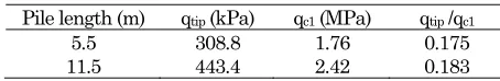
Table 4. Tip Resistance Ratio
Pile length (m) qtip (kPa) qc1 (MPa) qtip /qc1
5.5 308.8 1.76 0.175
11.5 443.4 2.42 0.183
Another sub-approach is to calculate the ratio of the side resistance to the cone penetration resistance. The ratio of the calculated side resistance to the average qc1 values is about 0.023 (≈ 1/44). This ratio is rather low compared to the maximum ratio for clay-silt with qc > 1 MPa which is 0.035 in the Dutch national practice [11].
The ratio of the lower bound calculated tip resistance to the average qc1 values in the pile tip area, or kc factor in the CFEM [2], is summarized in Table 4; the calculated kc factor ranges from 0.17 to 0.19. This calculated kc factor is significantly less than the CFEM recommended kc factor for clayey soil with qc = 1–5 MPa which is 0.35. It is noted that the CFEM recommended kc factor for silty soils qc < 5 MPa is 0.40. It can be seen that the lower bound calculated tip resistance indicates that the CFEM recommend-dations appear to be very high, but this issue warrants further evaluation as these piles behaved most likely as friction piles.
The lower bound calculated tip resistance is low compared to other recommendations. The French practice [12] recommends qtip/qc of 0.55 for driven piles in clay-silt. Jardine et al. (in [13]) recommends qtip/qc of 0.8–1.0 depending on loading conditions for driven piles in clay-silt. Again, this significant difference suggests that further evaluation is needed. In addition, the ratio of the model elastic modulus to the average qc1 values is about 10. This calculated ratio is low relative to the ratio suggested by Poulos [14], which ranges from 15 to 21. This significant difference in the modulus/qc1 ratio needs to be examined further.
Conclusions
Two (2) pile axial load tests were performed in a site with predominantly silt-clay soil. The piles were 5.5 m long and 11.5 m long 250-mm-square-concrete precast piles. The load-settlement curves of both piles suggested that the ultimate capacity of the piles were achieved. These unique features (axial load tests of piles with different lengths and load-settlement curves indicating failures) provided insights into the behavior of pile foundation in this type of soil. The axial load tests were subsequently back-analyzed using an axisymmetric finite element model. In the back-analyses, the soil properties in the model, using the cone penetration resistance as the reference, were adjusted so that the numerical load-settlement curves matched the actual curves.
The key observations from the comparison include the following: 1) the normalized cone penetration resistance qc1 provides a basis for better curve fitting and 2) the recommendation in the CFEM and in the Belgian national practice related to the side resistance appears to be applicable for this particular clay-silt soil, but that in the Dutch national practice appears to be relative too high for use at this site. Issues that warrant further evaluation include: 1) the tip resistance and 2) the soil modulus.
References
1. Tjandra, D. and Wulandari, P.S., Pengaruh Elektrokinetik terhadap Daya Dukung Pondasi Tiang di Lempung Marina, Civil Engineering Dimension, Vol. 8(1), 2006, pp.15–19.
2 Canadian Geotechnical Society, Canadian Foundation Engineering Manual, BiTech Publishers, Richmond, 1992.
3 Mayne, P.W., Cone Penetration Testing – A Synthesis of Highway Practice (NCHRP Synthesis 368), Transportation Research Board, Washington, D.C., 2007.
4 American Society for Testing and Materials, Standard Test Method for Mechanical Cone Penetration Tests of Soil (D3441), Annual Book of Standards, Vol. 04.08, Philadelphia, 2008.
5 Robertson, P.K., Soil Classification using the Cone Penetration Test, Canadian Geotechnical Journal, Vol. 27(1), 1990, pp.151-158.
6 Liao, S.C. and Whitman, R.V., Overburden Correction Factors for SPT in Sand, J. Geotechnical Engineering, ASCE, Vol. 114(4), 1986, pp.373-377.
7 American Society for Testing and Materials, Standard Test Method for Piles under Static Axial Compressive Load (D1143), Annual Book of Standards, Vol. 04.08, Philadelphia, 2008. 8 Hirany, A. and Kulhawy, F.H., Conduct and
Interpretation of Load Tests on Drilled Shaft Foundation: Detailed Guidelines (Report EL-5915 (1)), Electric Power Research Institute, Palo Alto, 1998.
9 Brinkgreve, R.B.J., PLAXIS 2D–Version 8, Balkema, Rotterdam, 2002.
11 Everst, H.J. and Luger, H.J., Dutch National Codes for Pile Design. Proc. ERTC3 Seminar– Design of Axially Loaded Piles European Practice, Brussels, 1997, pp. 243-265.
12 Bustamante, M. and Frank, R. 1997. Design of Axially Loaded Piles–French Practice. Proc. ERTC3 Seminar–Design of Axially Loaded Piles European Practice, Brussels, 1997, pp.161-175.
13 Poulos, H.G., Carter, J.P., and Small, J.C., Foundations and Retaining Structures–Research and Practice, Proc. 15th International Conference Soil Mechanics & Geotechnical Engineering, Istanbul, Vol. 4, 2001, pp.2527-2606.