UNDERSTANDING THE BEHAVIOUR OF CONTAMINATION SPREAD IN NAGARJUNA
SAGAR RESERVOIR USING TEMPORAL LANDSAT DATA
K. Tarun Teja a, *, K. S. Rajan a
a Lab for Spatial Informatics, IIIT-Hyderabad, Hyderabad, 500032, INDIA - [email protected], [email protected]
Commission VIII, WG VIII/4
KEY WORDS: Nutrient Pollution, Nagarjuna Sagar reservoir, Remote sensing, LANDSAT, Inland water bodies.
ABSTRACT:
LANDSAT images are used to identify organic contaminants in water bodies, but, there is no enough evidence in present literature that LANDSAT is also good in identifying a mixture of organic and mineral contaminants such as agricultural waste. The focus of this paper is to evaluate the effectiveness of LANDSAT imagery to identify organic and mineral contamination (OMC) and to identify spread extent variations of pollution over the season/year in the Nagarjuna Sagar (NS) reservoir using only satellite images. A new band combination is proposed in order to detect OMC, because existing formulae based on band ratio proved to be inadequate in detecting the contamination in NS. Difference in reflectance values of Red and Green channel of an image helps clearly distinguish clear water from OMC water. This procedure was applied over LANDSAT data of the calendar years 2008, 2014 and 2015 to understand the contamination spread pattern through the reservoir. Results show that contamination is following a similar pattern over these calendar years. In January contamination starts at inlets and by May contamination spreads to almost 90% of the reservoir when the total area of water spread is also reduced by half. Contamination spread is low during the monsoonal period of June to September due to heavy inflow and heavy outflow of waters from NS reservoir. Post monsoon NS is contaminated again because of heavy inflow of runoffs from neighboring land use and limited water outflow. This contamination spread pattern matches the agricultural seasons and fertilizer application pattern in this region, indicating that agricultural use of fertilizers could be one of the primary causes of contamination for this waterbody.
1. INTRODUCTION
Natural and anthropogenic reasons are two major causes of water resource contamination; anthropogenic factors such as high urbanization, industrialization and intensive agricultural practices have increased and accelerated the contaminants that are being delivered to water resources, so, water bodies are not able to recover from these contaminations naturally (Rodriguez et al., 2007). While the point source such as industrial and urban waste can be identified and handled for reduction in contamination, the non-point contamination sources such as agriculture runoffs are major problem throughout the world as these sources are hard to trace (Zeng et al., 2009, Linxu et al., 2010, Xue et al., 2008). Contaminants from these sources are both organic or inorganic. Okache et al., (2015), Zhang et al, (2009) and Dosskey, (2001) discussed the adverse effects of these type of contaminants and how uncontrolled contamination results in decline of drinking water quality, human and animal health issues, sedimentation and degradation of aquatic ecosystem.
Dauer et al., (2000) emphasizes that land use surrounding the water body influences the type of contaminants contaminating the water body; contaminants coming from industrial outlets and houses are continuous while contaminants from agricultural land use are periodic (Vega et al., 1998); so, understanding the behavior of spread of contaminates in water body will provide insight on what type of contaminants are contaminating the water and their source.
Works have been done to identify contamination in water bodies using onsite measurements, for example, the work done by Jinaguang et al., (2005) using field hyperspectral data. These kind of studies are not always feasible due to high cost, effort and time in sample collection and chemical analysis. So, remote analysis is potentially the most preferred way of monitoring the water bodies. Shao Meng et al., (2003), Wu et al., (2010), He et al., (2012), Xiaoyi et al., (2010) devised methods that merge field data and remote analysis using sensors, wireless transmitters and analysis at remote locations, but this needs heavy investment and continuous maintenance. Remote analysis using Satellite imagery is another very efficient and effective way to monitor contaminants in water body. Chang et al., (2014), Palmer et al., (2015), Kutser, (2009) reviewed the sensors available, possibilities and methods available to detect contaminants in inland water bodies and agreed that using satellite imageries to study inland water contamination is indeed one of the best available options.
NIR bands are used. Matthews et al., (2011) work also emphases that green to red band ratios were used by many past studies to detect contaminants in water body.
Most of the work in inland water body contamination detection was done outside tropical regions by using measurements calculated in those locations. In earlier discussion it was made clear that LANDSAT images are well suited for this kind of study after some degree of pre-processing, but, it should be taken into consideration that the existing literature and work on water contamination detection was mainly done using sensors that have higher radiometric resolution such as MODIS and MERIS. Kutser, (2012) agrees that LANDSAT has low radiometric sensitivity and thus the results given by this sensor may not be accurate in case of LANDSAT 4, 5, and 7 when their method of band ratio was used. Matthews et al., (2011) mentioned that MERIS and MODIS are better suitable for inland water body studies, because, these sensors have higher radiometric sensitivity when compared to the older data of LANDSAT. The availability of LANDSAT 8 with 10-bit radiometric information in those images may prove to be a good candidate for such studies. But, this sensor has not yet been tested in this environment, hence, this paper attempts at evaluating the use of LANDSAT 8 for such studies in large water bodies.
All the above studies tried or explained methods to detect a single type of contamination such as CDOM, TSS, chl-a or either organic or inorganic content but not in an environment where there is mixture of organic and mineral contaminants that are usually caused by agricultural runoffs. This studies purpose is to develop a method that helps to detect this kind of contamination. If we assume that the major contamination is agricultural runoff, then the method should also help detect the seasonal variations due to such anthropogenic activity with or without lag. This may further help to understand the interaction between the contamination source and pollution in water body. This study is an effort to fill these existing gaps in OMC detection using LANDSAT and understand how a contamination is spreading in the water body.
1.1 Study area
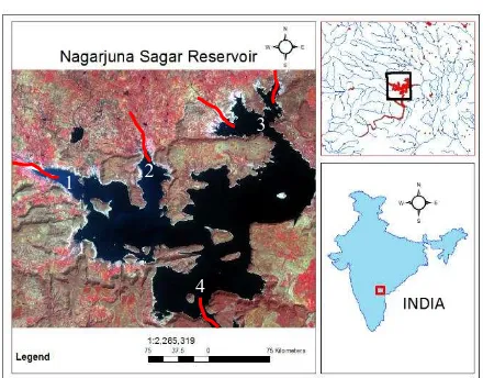
Nagarjuna Sagar (NS) reservoir which is situated between 16o 27’
11”N to 16o 40’19”N and 079o 02’08” E to 079o 20’50”E is being used as study area for this study. NS and its neighborhood is shown in Fig 1. NS is one of the biggest reservoir in India and it is used for irrigation, drinking water supply, water storage, generating hydroelectricity and also a very important neighborhood for land and fresh water ecosystem. NS is surrounded by Eastern Ghats on east and south side which also is part of NS-Srisailam Tiger reserve and serves as water source for forest animals and also is a very good tourist spot too. Keeping in mind that this water body is used in so many ways its becomes a necessity to check the water quality of the reservoir regularly.
2. Materials and Methods
LANDSAT 8 2014, 2015 and LANDSAT 5 images of years 2008 were downloaded for the study area, preferably cloud free images. There are only four, six and eight images for 2008, 2014 and 2015 respectively. Total eighteen images of size 994 x 767 were processed and analyzed in this study. Fig 2 shows the flowchart of this study and all the images were processed in similar procedure.
2.1 Data Normalization
This study uses LANDSAT 5 and 8 images. Even though there is similarity in band widths it is hard to compare the DN values due to changes in solar angle and satellite angles, and sometimes because of data format itself. DN values represent the data in percentages and since the data has different bit level it becomes difficult to compare data sets from these two data sources. Converting the DN values to irradiance reflectance values helps to standardizes the data and will make the comparison meaningful. Equation 1 and 2 are used to convert DN values of LANDSAT to top of atmosphere reflectance (TOAR) values (http://landsat.usgs.gov/Landsat8_Using_Product.php).
�= ����+ � (1)
Where � = TOA spectral radiance (Watts/ (m2 × srad × µm) � = Band - specific Multiplicative rescaling factor
���� = Quantized and calibrated standard Figure 1. Nagarjuna Sagar reservoir. Points 1,2,3 and 4 are
major inlets to this reservoir
1 2
3
4
Satellite Image
DN to Top of Atmosphere reflectance values
TOAR (Green – Red)
Calculate area of contamination spread of each class
Figure 2: Flowchart showing the procedure followed for this study
product pixel values (DN)
�� = Band – specific additive rescaling factor
��′= �����+ �� (2)
Where ��′ = TOA planetary radiance (Watts/ (m2 × srad × µm) � = Band - specific Multiplicative rescaling factor
���� = Quantized and calibrated standard product pixel values (DN)
�� = Band – specific additive rescaling factor
2.2 Detecting Contaminants
Band ratios that were used in other studies were tried first but, they did not produce satisfactory results. So, there was a need to develop a new method. Difference between TOAR Green and Red band was performed. The reason why band difference was used rather than band ratio is that the reflectance from Red channel is much higher than in Green channel if the water body is contaminated by organic matter. In such a scenario, band ratio between these two bands would result in values that are way less than 1 and standard deviation of the data will be very less. This effect coupled with low radiometric sensitivity of LANDSAT will make it difficult to differentiate between contamination and clear water. In addition, this method was developed only for CDOM detection but not OMC. In case of OMC the assumption is that the reflectance in Green band is more than that in Red channel. Hence, band difference between Green and Red channels would provide necessary pixel values which are positive and the data has better pixel variation to clearly identify the OMC contamination. Resulting image from this approach provides a single band image which clearly demarcates the contaminated regions of NS. To represent the contaminated regions and to calculate statistics the image has been classified using threshold values.
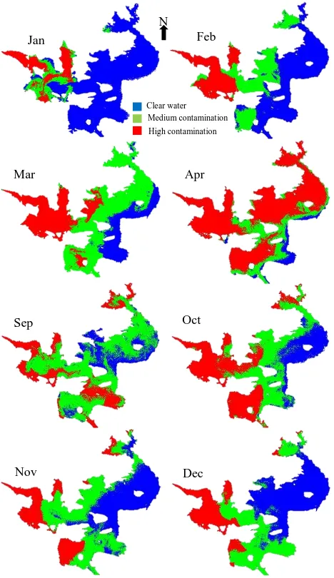
Threshold values are unique to an image and had to be calculated for every image. Threshold values represent the boundary between the contaminated and non-contaminated parts of the water body; these boundaries are selected using visual inspection. For example, Fig 3 demonstrates how the contamination is spreading in January, February, March, April, September, October, November and December moths of year 2015. Red color indicates High contamination area, Green color indicates medium contamination area and Blue color indicates the area where the contamination is low or is almost clear water. Then this classified image was corrected for errors using visual inspection of the original dataset.
3. Results and Discussion
Table 1 shows the area of contamination spread in Sq. Km and Table 2 shows contamination spread in percentage. Fig 1 shows the inlets from which the contaminants enter the water body mainly. While points 1, 2 and 3 on the figure show inlet channels from the neighborhood, point 4 indicates primary river inlet channel to the reservoir. From fig 1 and 3 it can be observed that contamination is spreading from the inlets 1, 2 and 3. Also the least amount of contamination can be observed in January and it keeps increasing and spreading across the reservoir. April and May months see the highest amount of contamination with almost 90% of the reservoir being contaminated. Table 1 and 2 can be used as reference here to see that April and May months are highly polluted months in all the years under study due to accumulation of contaminants and
reduced or no inflow of water leads to no dilution during this period, as it is the peak of summer. Images from June to September are not used due to high cloud cover as this is the monsoonal period around the tropic of cancer. During September to December it can be clearly observed that contamination spread is fluctuating. This can be attributed to two factors – while the increase in the contamination is due to immediate runoff from surrounding agricultural land use draining into the water bodies with the coming to an end of the main cropping season, the decrease may be due to increased water inflow into the reservoir due to North-east returning monsoon.
4. Potential cause of contamination
Year Month High Medium Nil Total water spread area
2008 Jan 57.01 9.98 84.27 151.2 Figure 3. Classification results showing the spread of
contaminations in NS from Jan to Dec in 2015.
Jan Feb
Mar Apr
Sep Oct
Nov Dec
N
Feb 79.13 34.77 36.55 150.4
Table 1. spread of contamination in Nagarjuna Sagar reservoir in Sq. Km
Table 2. spread of contamination in Nagarjuna Sagar reservoir in percentage
NS is surrounded by agricultural fields. Agriculture is one of most practiced land use in tropical countries such as India and is one of the best source of income (Directorate of Economics and Statistics of India, 2014). Heavy usage of fertilizers and pesticides is part of agricultural practices in India to boost production and maintain the income. The excess amount of unutilized nutrients and chemicals are drained into streams and waterbodies nearby. Agarwal, (1999) and Carpenter et al., (1998) reviewed the effect of agriculture practices on water quality and stated that nutrient pollution from agricultural area is a dangerous problem and leads to eutrophication. NS is surrounded by agricultural fields and hence
312 306
Jan Feb Mar Apr May June July Aug Sep Oct Nov Dec Urea utilization in 2008 in Andhra Pradesh
Figure 4. Urea added to agricultural fields during 2008 and 2013 in Andhra Pradesh.
Jan Feb Mar Apr May June July Aug Sep Oct Nov Dec Urea utilization in 2013 in Andhra Pradesh
38
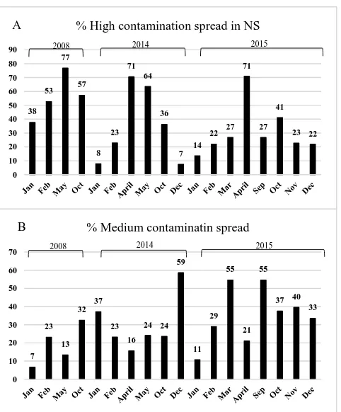
% High contamination spread in NS
2008 2014 2015
Figure 5. Percentage High, Medium contamination spread during 2008, 2014 and 2015
A
there is a high possibility that nutrient contamination is happening to NS. Fig 4 shows the amount of fertilizers used during year 2008 and 2013 in 100 billion Megatons in the state of Andhra Pradesh-NS is entirely located within its administrative boundaries. India is third largest producer of fertilizer and second largest consumer of fertilizers for its needs, so, these number will only increase in the future.
Using the values from Table 2, graphs in Fig 5 were generated to show the overall variations in contamination spread in 2008, 2014 and 2015, A denotes percentage of Highly contaminated area and B denotes percentage of medium contaminated areas in 2008, 2014 and 2015. Fig 5A indicates that the contamination in NS is following the fertilizer utilization pattern of 2008 and 2013 with 3 to 4 months of lag. January to May the contamination keeps on increasing as fertilizers are carried into the reservoir, and it is coupled with the reduction in water area spread. This helps in increasing the contamination spread area. Post September, the rise is due to end of Kharif (rainfed) cropping season and the land being washed out. Similarly, medium level contamination details from Fig 5B show that this type of contamination also follows the fertilizer usage pattern, but, spreads in larger area and undergoes heavy transport due to movement of water.
5. Conclusion
Difference in reflectance values of Red channel and Green channel is proposed as a new method to detect OMC in very large water bodies. This method gives good results when detecting OMC from very large water bodies such as NS, located in tropical regions, using LANDSAT 5, and 8. This study reveals that NS is highly contaminated in April and May. Contamination spread is following a pattern that matches the agricultural fertilizer usage practices, and it can be said that NS is getting contaminated because of agricultural runoffs which are high in nutrients. validation of this work by measuring the concentration of these contaminants during the satellite overpass will help in establishing this method as a preferred procedure when checking for agricultural contaminants in very large water bodies. There is a need to explore further to understand how this procedure will perform when other radiometric insensitive data is used. Effectiveness of this procedure on other lager water bodies over different regions need to be studied; because a generalized method to detect OMC is more preferred to developing unique algorithms for specified water body or a set of water bodies. These are beyond the scope of current study but are set as future goals to be pursued later.
6. References
Agarwal, G. D., 1999. Diffuse agricultural water pollution in India. Water Science & technology, 39(3), pp. 33-47.
Carpernter, S. R. Caraco, N. F. Correll, D. L. Howarth, R. W. Sharpley, A. N. and Smith, V. H., 1998. Non point pollution of surface waters with phosphorus and nitrogen. Ecological Applications, 8(3), pp. 559-568.
Dosskey, G. M., 2001. Towards quantifying water pollution abatement in response to installing buffers on crop land. Environmental Management, 28(5), pp. 577-598.
Dauer, D. M. Ranasinghe, J. A. Weisberg, S. B., 2000. Relationships between benthic community condition, water quality, sediment quality, nutrient loads, and land use patterns in Chesapeake Bay. Estuaries, 23(1), pp. 80-96.
Department of Fertilizers, Ministry of Chemicals and Fertilizer, Government of India., 2014. “Indian fertilizer scenario 2014” http://fert.nic.in/page/publication-reports (5 April. 2016).
Department of Fertilizers, Ministry of Chemicals and Fertilizer, Government of India., 2015, “Indian fertilizer scenario 2013”. http://fert.nic.in/page/publication-reports (5 April. 2016).
Directorate of Economics & Statistics, Department of Agriculture & Cooperation, Ministry of Agriculture, Government of India., 2015. “Pocket book of Agricultural Statistics 2014” http://eands.dacnet.nic.in/PDF/Pocket-Book2014.pdf (5 April. 2016).
He, D. and Zhang, L. X., 2012. The water quality monitoring system based on WSN: 2nd International Conference on Consumer Electronics and Communications and Networks (CECNet), Yichang, pp. 3661-3664.
Kutser, T., 2012. The possibility of using the LANDSAT image archive for monitoring long time trends in coloured dissolved organic matter concentration in lake waters. Remote Sensing of Environment, 123, pp. 334-338.
Matthews, M. W., 2011. A current review of empirical procedures of remote sensing in inland and near – coastal transitional waters. International Journal of Remote Sensing, 32(21), pp. 6855-6899.
Okache, J. Haggett, B. Maytum, R. Mead, A. Rawson D. and Ajmal, T., 2015. Sensing fresh water contamination using fluorescence methods: SENSORS, 2015 IEEE, Busan, pp. 1-4.
Odermatt, D. Gitelson, A. Brando, V. E. and Schaepman, M., 2012. Review of constituent retrieval in optically deep and complex waters from satellite imagery. Remote Sensing of Environment, 118, pp. 116-126.
Palmer, S. C. J. Kutser, T. Hunter, P. D., 2015. Remote sensing of inland waters: Challenges, progress and future directions. Remote Sensing of Environment, 157, pp. 1-8.
Rodruguez, W. August, P. V. Wang, Y. Paul, J. F. Gold, A. and Rubinstein, N., 2006. Empirical relationships between land use/cover and estuarine condition in the northeastern United States. Landscape Ecol, 2007, 22, pp. 403-417.
Shao-meng, Q. Qi-zhong, L. and Xue, C., 2003. An improved method of spectral unmixing and its application in water pollution monitoring: Geoscience and Remote Sensing Symposium, IGARSS '03. Proceedings, 2003 IEEE International, vol.4, pp. 2456-2458.
U.S. Geological Survey, 2013, “LANDSAT 8 Handbook”,
http://landsat.usgs.gov//l8handbook_section5.php (15 April. 2016) .
Wang X. Jun, D. Zaiwen, L. Xiaoping, Z. Suoqi, D. Zhiyao, Z. Miao, Z., 2010. The lake water bloom intelligent prediction method and water quality remote monitoring system: Sixth International Conference on Natural Computation (ICNC) 2010, Yantai, Shandong, pp. 3443-3446.
Wu, Q. Liang, Y. Sun, Y. Zhang, C. and Liu, P., 2010. Application of GPRS technology in water quality monitoring system: World Automation Congress (WAC), Kobe, pp. 7-11.
Xue, L. Hao, Z. Huo, T. and Li, D., 2008. The Distributed Stochastic Monitoring and Modeling on Non-Point Source Pollution and Water Ecosystem Health Assessment: The 2nd International Conference on Bioinformatics and Biomedical Engineering, ICBBE 2008. Shanghai, pp. 4263-4266.
Zeng, H. Zheng, D. Yang, S. Wang, X. Gao, Y. and Fu, Z., 2009. RS & GIS based assessment of adsorptive non-point source pollution in eucalyptus and rubber plantation at the water source area of Hainan: Geoscience and Remote Sensing Symposium, 2009 IEEE International, IGARSS 2009, Cape Town, pp. III-152-III-155.