CONDITIONAL RANDOM FIELDS FOR LIDAR POINT CLOUD CLASSIFICATION IN
COMPLEX URBAN AREAS
J. Niemeyer∗
, F. Rottensteiner, U. Soergel
Institute of Photogrammetry and GeoInformation, Leibniz Universit¨at Hannover D-30167 Hannover, Germany, (niemeyer, rottensteiner, soergel)@ipi.uni-hannover.de
Commission III/4
KEY WORDS:Classification, Urban, LiDAR, Point Cloud, Conditional Random Fields
ABSTRACT:
In this paper, we investigate the potential of a Conditional Random Field (CRF) approach for the classification of an airborne LiDAR (Light Detection And Ranging) point cloud. This method enables the incorporation of contextual information and learning of specific relations of object classes within a training step. Thus, it is a powerful approach for obtaining reliable results even in complex urban scenes. Geometrical features as well as an intensity value are used to distinguish the five object classesbuilding,low vegetation,tree, natural ground, andasphalt ground. The performance of our method is evaluated on the dataset of Vaihingen, Germany, in the context of the ’ISPRS Test Project on Urban Classification and 3D Building Reconstruction’. Therefore, the results of the 3D classification were submitted as a 2D binary label image for a subset of two classes, namelybuildingandtree.
1 INTRODUCTION
The automated detection of urban objects from remote sensing data has become an important topic in research in photogram-metry and remote sensing. The results are necessary to derive object information for applications such as the generation of 3D city models for visualization and simulations. Data acquired by an airborne LiDAR sensor are especially suitable for this task be-cause they directly describe the object surface in 3D. The core task resolved in this context is the classification of such a point cloud. However, in dense urban areas reliable point labeling is a challenging task due to complex object structure and the high variability of object classes (e.g. buildings, roads, trees, and low vegetation) appearing in this kind of scene. In such a man-made environment different objects usually have a specific kind of re-lations, which can be utilized in a contextual classification to dis-tinguish multiple object classes simultaneously. Thus, the quality of classification can be improved by incorporating context infor-mation compared to approaches only classifying each point inde-pendently from its neighbors.
A Conditional Random Field (CRF) is a generalization of a Mar-kov Random Field (MRF) and provides a flexible statistical clas-sification framework for modeling local context. Originally in-troduced by Lafferty et al. (2001) for labeling one-dimensional sequence data, it has become increasingly popular in computer vision since the approach was adapted to the classification of im-ages by Kumar and Hebert (2006). Some investigations were carried out in the field of remote sensing. For instance, Wegner (2011) analyzes the potential of CRF for building detection in op-tical airborne images. However, there is only a small amount of work dealing with LiDAR point clouds.
Some initial applications of contextual classification can be found related to robotics and mobile laser scanning utilizing terrestrial LiDAR point clouds. Anguelov et al. (2005) performed a point-wise classification on terrestrial laser scans using a simplified subclass of Markov Models, called Associative Markov Networks (AMNs) (Taskar et al., 2004), which encourage neighboring points to belong to the same object class. However, AMNs have some
∗Corresponding author
drawbacks: Small objects cannot be detected correctly due to over-smoothing. In the approach presented by Lim and Suter (2009) a terrestrial point cloud acquired by mobile mapping is processed in two steps. Firstly, they over-segment the data and secondly they perform a segment-wise CRF classification. Where-as this Where-aspect helps to cope with noise and computational com-plexity, the result heavily depends on the segmentation, and small objects with sub-segment size cannot be detected. Shapovalov et al. (2010) investigated the potential of CRFs for the classifica-tion of airborne LiDAR point clouds. They improved the draw-backs of an AMN by applying a non-associative Markov Net-work, which is able to model typical class relations such as ’tree is likely to be above ground’. These interactions represent addi-tional context knowledge and may improve classification results. Similar to the approach described before, the authors applied a segment-based classification; hence, it is limited due to its de-pendence on the segmentation.
In our previous work (Niemeyer et al., 2011) we introduced a point-wise CRF classification of airborne full-waveform LiDAR data. This approach requires higher computational costs, but en-ables the correct detection of smaller objects. Each point is linked to points in its geometrical vicinity, which influence each other in the classification. All labels of the entire point cloud are deter-mined simultaneously. The three object classesground,building, andvegetationwere distinguished. However, we applied a simple model for the interactions, penalizing the occurrence of different class labels of neighboring points, if the data did not indicate a change. Moreover, the decision surface in feature space was mod-eled by a linear function, which may not separate the clusters in a good way.
a binary label image is generated by rasterization for each class of interest. The boundaries of objects are smoothed by apply-ing a morphological filter afterwards. Our results are evaluated in the context of the ’ISPRS Test Project on Urban Classification and 3D Building Reconstruction’ hosted by ISPRS WG III/4, a benchmark comparing various classification methods based on aerial images and/or LiDAR data of the same test site.
The next section presents our methodology including a brief de-scription of the CRF. After that, Section 3 comprises the evalua-tion of our approach as well as discussions. The paper concludes with Section 4.
2 METHODOLOGY
2.1 Conditional Random Fields
It is the goal of point cloud classification to assign an object class label to each 3D point. Conditional Random Fields (CRFs) pro-vide a powerful probabilistic framework for contextual classifi-cation and belong to the family of undirected graphical models. Thus, data are represented by a graphG(n,e)consisting of nodes nand edgese. For usual classification tasks, spatial units such as pixels in images or points of point clouds can be modeled as nodes. The edgeselink pairs of adjacent nodesniandnj, and
thus enable modeling contextual relations. In our case, each node ni ∈ncorresponds to a 3D point and we assign an object class
labelyibased on observed dataxin a simultaneous process. The
vectorycontains the labelsyifor all nodes and hence has the
same number of elements liken.
In contrast to generative Markov Random Fields (MRFs), CRFs are discriminative and model the posterior distribution P(y|x)
directly. This leads to a reduced model complexity compared to MRFs (Kumar and Hebert, 2006). Moreover, MRFs are re-stricted by the assumption of conditionally independent features of different nodes. Theoretically, only links to nodes in the imme-diate vicinity are allowed in this case. These constraints are re-laxed for CRFs, consequently more expressive contextual knowl-edge represented by long range interactions can be considered in this frameworks. Thus, CRFs are a generalization of MRFs and model the posterior by In Eq. 1,Niis the neighborhood of nodenirepresented by the
edges linked to this particular node. Two potential terms, namely theassociation potentialAi(x, yi)computed for each node and
theinteraction potentialIij(x, yi, yj)for each edge are modeled
in the exponent; they are described in Section 2.4 in more de-tail. The partition functionZ(x)acts as normalization constant turning potentials into probability values.
2.2 Graphical Model
In our framework, each graph node corresponds to a single Li-DAR point, which is assigned to an object label in the classifica-tion process. Consequently, the number of nodes innis identical to the number of points in the point cloud. The graph edges are used to model the relations between nodes. In our case, they link to the local neighbor points in object space. A nearest neighbor search is performed for each pointni to detect adjacent nodes
nj ∈Ni. Each point is linked to all its neighbors inside a
verti-cal cylinder of a predefined radiusr. Using a cylindrical neigh-borhood enables to model important height differences, which
are not captured in a spherical vicinity (Shapovalov et al., 2010; Niemeyer et al., 2011). The cylinder radiusrdetermines the size ofNiand thus should be selected related to the point density; a
tradeoff between number of edges and computational effort must be chosen (Section 3.1).
2.3 Features
In this research, only LiDAR features are utilized for the classi-fication of the point cloud. A large amount of LiDAR features is presented in Chehata et al. (2009). They analyzed the relative importance of several features for classifying urban areas by a random forest classifier. Based on this research, we defined 13 features for each point and partially adapted them to our specific problem.
Apart from theintensity value, all features describe the local ge-ometry of point distribution. An important feature isdistance to ground (Chehata et al., 2009; Mallet, 2010), which models each point’s elevation above a generated or approximated terrain model. In the original work, this value is approximated by us-ing the difference of the trigger point and the lowest point ele-vation value within a large cylinder. The advantage of this ap-proximation is that no terrain model is necessary, but this as-sumption is only valid for a flat terrain and not for hilly ground. We adapted the feature, but computed a terrain model (DTM) by applying the filtering algorithm proposed in Niemeyer et al. (2010). The additional features consider a local neighborhood. On the one hand, a spherical neighborhood search captures all points within a 3D-vicinity; on the other hand, points within a vertical cylinder centered at the trigger point model the point dis-tribution in a 2D environment. By utilizing thepoint density ratio (npts,sphere/npts,cylinder), a useful feature indicating vegetation
can be computed. Points within a sphere are used to estimate a local robust 3D plane. Thesum of the residualsis a measurement of the local scattering of the points and serves as feature in our experiment. Thevariance of the point elevationswithin the cur-rent spherical neighborhood indicates whether significant height differences exist, which is typical for vegetated areas and build-ings. The remaining features are based on the covariance matrix set up for each point and its three eigenvaluesλ1,λ2, andλ3. The local point distribution is described by eigenvalue-based features such aslinearity,planarity,anisotropy,sphericity, andsum of the eigenvalues. Equations are provided in Table 1.
Eigenvalues λ1≥λ2≥λ3
After computation, the feature values are not homogeneously sca-led due to the different physical interpretation and units of these features. In order to align the ranges, a normalization of each fea-ture for all points of a given point cloud is performed by subtract-ing the mean value and dividsubtract-ing by its standard deviation. Many features depend on the eigenvalues, which leads to a high correla-tion. Thus, a principal component analysis (PCA) is performed. Nine of the obtained uncorrelated 13 features (maintaining 95 % of information) are then used for CRF-based classification. In a CRF, each node as well as each edge is associated to a feature vector. Since each 3D LiDAR point represents a single nodeni,
we use the 9 features described above to define that node’s feature vectorhi(x). Edges model the relationship between each pointni
absolute difference between the feature vectors of both adjacent nodes to compute the interaction feature vector
µij(x) =|hi(x)−hj(x)|. (2)
2.4 Potentials
The exponent of Eq. 1 consists of two terms modeling different potentials.Ai(x, yi)links the data to the class labels and hence it
is calledassociation potential. Note thatAimay potentially
de-pend on the entire datasetxinstead of only the features observed at nodeniin contrast to MRFs. Thus, global context can be
inte-grated into the classification process.Iij(x, yi, yj)represents the
interaction potential. It models the dependencies of a nodenion
its adjacent nodesnjby comparing both node labels and
consid-ering all the observed datax. This potential acts as data-depended smoothing term and enables to model the incorporation of contex-tual relations explicitly. For both,AiandIij, arbitrary classifiers
can be used. We utilize a generalized linear model (GLM) for all potentials. A feature space mapping based on a quadratic feature expansion for node feature vectorshi(x)as well as the interaction
feature vectorsµij(x)is performed as described by Kumar and Hebert (2006) in order to introduce a more accurate non-linear decision surface for classes within the feature space. This is in-dicated by the feature space mapping functionΦand improves the classification compared to our previous work (Niemeyer et al., 2011), in which linear surfaces were used for discriminating object classes. Each vectorΦ(hi(x))andΦ(µij(x))consists of
55 elements after expansion in this way.
The association potentialAidetermines the most probable label
for a single node and is given by
Ai(x, yi=l) =wTl ·Φ(hi(x)), (3)
wherehi(x)is a feature vector of nodenicomputed from datax
andwlis a vector of feature weights for a certain classl. In the
training step there is one such weight vector learned per class. The interaction potentialIijmodels the influence of each point’s
neighborhood to the classification process. Therefore, a feature vectorµij(x)is computed for each edge in the graph and multi-plied to an edge weight vectorvl,k, which depends on the label
configuration of both adjacent nodesniandnj:
Iij(x, yi=l, yj=k) =vTl,k·Φ(µij(x)). (4)
There is one weight vectorvl,kfor each combination of classes
landk, which are also determined in the training stage. In our previous work (Niemeyer et al., 2011), different class labelsland kwere penalized, becauseIij(x, yi, yj)was modeled to be
pro-portional to the probabilityP(yi =yj|µij(x)). For the current
research, this potential is enhanced and is proportional to the joint probabilityP((yi, yj)|Φ(µij(x))). Thus, there is a probability
for each label configuration. Trained in a learning step, certain class relations are modeled to be more probable than others are. For instance, a point assigned to classbuildingis not likely be surrounded by points belonging towater. This advanced infor-mation is used to improve the quality of classification. Moreover, the degree of smoothing depends on the feature vectorµij(x).
For this reason, small objects are better preserved if there is suffi-cient evidence in the data, which is a major advantage in complex urban areas (Niemeyer et al., 2011).
2.5 Inference and Training
Exact inference and training is intractable in our application due to the fact that our graphG(n,e) is large and contains cycles. Thus, approximate methods have to be applied in both cases.
Loopy Belief Propagation (LBP) (Frey and MacKay, 1998) is a standard iterative message passing algorithm for graphs with cy-cles. We use it for inference, which corresponds to the task of determining the optimal label configuration based on maximizing P(y|x)for given parameters. The result is a probability value per class for each node. The highest probability is selected according to the maximum a posteriori (MAP) criterion; the corresponding object class label obtaining the maximum probability is assigned to the point afterwards. For the classification, the two vectors wlandvl,k are required, which contain the feature weights for
association potential and interaction potential respectively. They are determined in a training step by utilizing a fully labeled part of a point cloud. All weights ofwlandvl,kare concatenated in
a single parameter vectorθ = [w1, . . .wc;v1,1. . .vc,c]T with
cclasses, in order to ease notation. For obtaining the best dis-crimination of classes, a non-linear numerical optimization is per-formed by minimizing a certain cost function. Following Vish-wanathan et al. (2006), we use the limited-memory Broyden-Fletcher-Goldfarb-Shanno (L-BFGS) method for optimization of the objective functionf =−logP(θ|x,y). For each iteration f, its gradient as well as an estimation of the partition function Z(x)is required. Thus, we use L-BFGS combined with LBP as implemented in M. Schmidt’s Matlab Toolbox (Schmidt, 2011). 2.6 Object generation
Since the result of the CRF classification is a 3D point cloud, we performed a conversion to raster space in order to obtain 2D objects for each class of interest. If any point was assigned to the trigger class, the certain pixel is labeled by value one and zero otherwise. A morphological opening is carried out to smooth the object boundaries in a post-processing step.
3 EVALUATION
3.1 Benchmark-Dataset
The performance of our method is evaluated on the LiDAR data-set of Vaihingen, Germany (Cramer, 2010), in the context of the ’ISPRS Test Project on Urban Classification and 3D Building Reconstruction’. The dataset was acquired in August 2008 by a Leica ALS50 system with a mean flying height of 500 m above ground and a 45◦
field of view. The average strip overlap is 30 %.
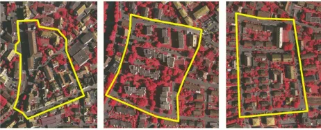
Figure 1: Test sites of scene Vaihingen. ’Inner City’ (Area 1, left), ’High-Riser’ (Area 2, middle) and ’Residental’ (Area 3, right) (Rottensteiner et al., 2011)
to learn the parameter weights (Section 2.5). For our experiments, a fully and manually labeled part of the point cloud with 93,504 points in the east of Area 1 was used.
According to the point density of this scene and based on the knowledge obtained in Niemeyer et al. (2011), we set the param-eter radiusrfor graph construction to 0.75 m for the following experiments, which results in 5 edges on average for each point. 3.2 Result CRF Classification
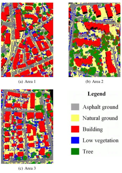
The original result of CRF classification is the assignment of an object class label to each LiDAR point. Hence, we obtain a la-beled 3D point cloud. Five classes were trained for this research: natural ground, asphalt ground, building, low vegetation, and trees. The results are depicted in Fig. 2.
(a) Area 1 (b) Area 2
(c) Area 3
Figure 2: 3D CRF-Classification results.
In general, our approach achieved good classification results. Vi-sual inspection reveals that the most obvious error source are points on trees incorrectly classified asbuilding. This is because most of the 3D points are located on the canopy and show similar features to building roofs: the dataset was acquired in August un-der leaf-on conditions, that is why almost the whole laser energy was reflected from the canopy, whereas second and more pulses within trees were recorded only very rarely (about 2 %). Most of our features consider the point distribution within a local neigh-borhood. However, for tall trees with large diameters the points on the canopy seem to be flat and horizontally located some me-ters above the ground, which usually hints for points belonging to building roofs. That is the reason for misclassification of some tree points tobuildings.
Due to missing complete 3D reference data, a quantitative evalu-ation of the entire point classificevalu-ation result cannot be performed.
Thus, we carry out an object-based evaluation in 2D as described in the Section 3.4.
3.3 Improvements of interactions & feature space mapping
In this research, two improvements for the CRF-framework are implemented: Firstly, the feature space mapping enables a non-linear decision surface in classification. Secondly, weights for all object class relations are learned. In order to evaluate the impact of these changes compared to the approach proposed in Niemeyer et al. (2011), we manually labeled the point cloud of Area 3 and carried out a point-wise validation based on this reference data. Therefore, the results are compared to a classification penaliz-ing different classes in the interaction model and without feature space mapping.
The enhanced CRF increases the overall accuracy by 5.38 per-centages and hence yields considerably more sophisticated re-sults. Table 2 shows the differences of completeness and correct-ness values in percentages obtained by the enhanced CRF classi-fication and the simpler model. Positive values indicate a higher accuracy of results obtained with the complex edge potential and feature space mapping. It can easily be seen, that all values are improved by introducing the complex method. Especially details such as small buildings or hedges are preserved (Fig. 3). To sum up, feature space mapping and modeling of all specific class rela-tions considerably improve the quality. Thus, it is worth the effort of learning more parameters in training.
Classes Completeness Correctness asphalt ground 6.04 6.55 natural ground 7.57 3.68
building 0.60 6.89
low vegetation 10.59 7.90
tree 4.81 1.39
Table 2: Comparison of enhanced CRF results and simpler model (differences of completeness and correctness values).
(a) simple model (b) enhanced model
Figure 3: Comparison of the results obtained by a simple and an enhanced CRF model. For instance, garages (white arrows) and hedges (yellow arrows) are better detected with the complex model.
3.4 Evaluation of 2D objects
order to smooth the fringed boundaries of the objects. These label images are then evaluated in the context of the ISPRS Test Project with the method described in Rutzinger et al. (2009) based on a reference for each class. The results are discussed in the follow-ing part.
3.4.1 Building: The first object class being analyzed is build-ing. Completeness and correctness values per-area are between 87.0 % and 93.8 %. The quality, which is defined as
Quality = 1/(1/Completeness + 1/Correctness−1), (5) reaches values from 79.4 % to 88.3 % (Table 3). It can be seen, that the quality of Area 1 is about 7 percentages below those ob-tained for the other two test sites. The corresponding classifi-cation results are depicted in Fig. 4. Yellow highlighted areas represent the true positives (TP), blue are false negative (FN) and red are false positive detections (FP). It becomes evident, that the majority of the building shapes were detected correctly. Thus, the approach works well for buildings.
Area 1 Area 2 Area 3 Completeness 87.0% 93.8% 93.8% Correctness 90.1% 91.4% 93.7% Quality 79.4% 86.2% 88.3% Table 3: Per-area accuracies of classbuilding
(a) Area 1 (b) Area 2 (c) Area 3
Figure 4: Pixel-wise result of classbuildings(yellow = TP, red = FP, blue = FN)
Most of the FPs are caused by tree areas wrongly misclassified asbuilding. This is due to the similar features, as mentioned before: the LiDAR points covering trees are mainly distributed on the canopy and not within the trees, which leads to a nearly horizontal and planar point distribution.
A very important feature for discriminating several classes such asgroundorbuilding roofis ’height above ground’ (Mallet, 2010). By utilizing a DTM for generating this feature in our application, buildingsandgroundcan be distinguished much better because of hilly ground. However, there are still some larger FN areas, e.g. in the center part of Area 1. This is due to the filtering pro-cess of the terrain model generation for this feature, because some buildings and garages situated next to other ground height levels could not be eliminated correctly. Thus, the height differences to ground are very small for these points and lead to a misclassifica-tion with object classground.
The evaluation on a per-object level for buildings in the three test sites is depicted in Fig. 5. It is a cumulative histogram show-ing the quality numbers for all buildshow-ings larger than the area cor-responding to the respective bin. Here, completeness, correct-ness and quality are computed separately for all area intervals of the abscissa. As shown in the figure, the accuracies of our method increase with larger object size. All buildings of Area 2 and 3 with an area larger than 87.5 m2 are detected correctly, whereas the quality in Area 1 reaches 100 % at objects larger
Figure 5: Evaluation of buildings on a per-object level as a func-tion of the object area (cumulative)
than 137.5 m2. The above-mentioned misclassification of small
regions with classtreecauses low correctness (and thus quality) values especially for Area 2.
3.4.2 Trees: The results of classtreevary considerably. Cor-rectness values are between 69.2 % and 77.0 %, whereas com-pleteness underperforms this with 41.4 % to 74.0 %. This finds expression in only reasonable quality values (Table 4). Especially in Area 1 low completeness values are obtained. As shown in Fig. 6, there are many undetected trees represented as FNs. These are mainly small trees, which were misclassified aslow vegetation due to the indistinct class definition oftreeandlow vegetationin the benchmark, which do not coincide in this case. In general, larger trees could be detected more reliably (Fig. 7). However, especially in Area 1 the cumulative histogram decreases for trees with a larger area due to misclassifications asbuilding.
Area 1 Area 2 Area 3 Completeness 41.4% 74.0% 55.9% Correctness 69.2% 73.1% 77.0% Quality 35.0% 58.2% 47.9% Table 4: Per-area accuracies of classtrees
(a) Area 1 (b) Area 2 (c) Area 3
Figure 6: Pixel-wise result of classtree
4 CONCLUSION AND OUTLOOK
In this work, we presented a context-based Conditional Random Field (CRF) classifier applied to complex urban area LiDAR sce-nes. Representative relations between object classes are learned in a training step and utilized in the classification process. Eval-uation is performed in the context of the ’ISPRS Test Project on Urban Classification and 3D Building Reconstruction’ hosted by ISPRS WG III/4 based on three test sites with different settings. The result of our classification is a labeled 3D point cloud; each point assigned to one of the object classesnatural ground, as-phalt ground,building,low vegetationortree. A test has shown that feature space mapping and a complex modeling of specific class relations considerably improve the quality. After obtain-ing a binary grid image with morphological filterobtain-ing for classes buildingandtree, which were taken into account in the test, the evaluation was carried out. In this case, the best results were ob-tained forbuildings, which could be detected very reliably. The classification results oftreevary considerably in quality depend-ing on the three test sites. Especially in the inner city scene many misclassifications occur, whereas the scenes consisting of high-rising buildings and residential areas could be classified reliably. Some of the small trees are classified aslow vegetationand hence are not considered in the benchmark evaluation leading to attenu-ated completeness values. In summary, it can be stattenu-ated that CRFs provide a high potential for urban scene classification.
In future work we want to integrate new features to obtain a robust classification even in scenes with low point densities in vegetated areas in order to allow a robust classification result and decrease the number of confusion errors with buildings. Moreover, multi-scale features taking larger parts of the environment into account might improve results. Finally, the classified points are grouped to objects in a simple way by 2D rasterization. They should be combined to 3D objects in the next steps by applying a hierarchi-cal CRF.
ACKNOWLEDGMENTS
The authors would like to thank Cl´ement Mallet for computing the point features used for classification. This work is funded by the German Research Foundation (DFG).
The Vaihingen data set was provided by the German Society for Photogrammetry, Remote Sensing and Geoinformation (DGPF) (Cramer, 2010):http://www.ifp.uni-stuttgart.de/dgpf/ DKEP-Allg.html(in German).
References
Anguelov, D., Taskar, B., Chatalbashev, V., Koller, D., Gupta, D., Heitz, G. and Ng, A., 2005. Discriminative learning of markov random fields for segmentation of 3d scan data. In: Proceed-ings of the 2005 IEEE Computer Society Conference on Com-puter Vision and Pattern Recognition (CVPR’05), Vol. 2, IEEE Computer Society, pp. 169–176.
Chehata, N., Guo, L. and Mallet, C., 2009. Airborne lidar feature selection for urban classification using random forests. In: In-ternational Archives of Photogrammetry, Remote Sensing and Spatial Information Sciences, Vol. XXXVIII, Part 3/W8, Paris, France, pp. 207–212.
Cramer, M., 2010. The DGPF-Test on Digital Airborne Camera Evaluation – Overview and Test Design. Photogrammetrie-Fernerkundung-Geoinformation 2010(2), pp. 73–82.
Frey, B. and MacKay, D., 1998. A revolution: Belief propagation in graphs with cycles. In: Advances in Neural Information Processing Systems 10, pp. 479–485.
Kumar, S. and Hebert, M., 2006. Discriminative random fields. International Journal of Computer Vision 68(2), pp. 179–201. Lafferty, J., McCallum, A. and Pereira, F., 2001. Conditional
random fields: Probabilistic models for segmenting and label-ing sequence data. In: Proceedlabel-ings of the 18th International Conference on Machine Learning, pp. 282–289.
Lim, E. and Suter, D., 2009. 3d terrestrial lidar classifications with super-voxels and multi-scale conditional random fields. Computer-Aided Design 41(10), pp. 701–710.
Mallet, C., 2010. Analysis of Full-Waveform Lidar Data for Ur-ban Area Mapping. PhD thesis, T´el´ecom ParisTech.
Niemeyer, J., Rottensteiner, F., Kuehn, F. and Soergel, U., 2010. Extraktion geologisch relevanter Strukturen auf R¨ugen in Laserscanner-Daten. In: Proceedings 3-L¨andertagung 2010, DGPF Tagungsband, Vol. 19, Vienna, Austria, pp. 298–307. (in German).
Niemeyer, J., Wegner, J., Mallet, C., Rottensteiner, F. and So-ergel, U., 2011. Conditional random fields for urban scene classification with full waveform lidar data. In: Photogram-metric Image Analysis (PIA), Lecture Notes in Computer Sci-ence, Vol. 6952, Springer Berlin / Heidelberg, pp. 233–244. Rottensteiner, F., Baillard, C., Sohn, G. and Gerke, M., 2011.
ISPRS Test Project on Urban Classification and 3D Building Reconstruction. http://www.commission3.isprs.org/ wg4/.
Rutzinger, M., Rottensteiner, F. and Pfeifer, N., 2009. A com-parison of evaluation techniques for building extraction from airborne laser scanning. IEEE Journal of Selected Topics in Applied Earth Observations and Remote Sensing 2(1), pp. 11– 20.
Schmidt, M., 2011. UGM: A Matlab toolbox for probabilis-tic undirected graphical models. http://www.di.ens.fr/ ~mschmidt/Software/code.html(Nov. 15, 2011). Shapovalov, R., Velizhev, A. and Barinova, O., 2010.
Non-associative markov networks for 3d point cloud classification. In: Proceedings of the ISPRS Commission III symposium -PCV 2010, International Archives of Photogrammetry, Remote Sensing and Spatial Information Sciences, Vol. 38/Part A, IS-PRS, Saint-Mand´e, France, pp. 103–108.
Taskar, B., Chatalbashev, V. and Koller, D., 2004. Learning asso-ciative markov networks. In: Proceedings of the 21st Interna-tional Conference on Machine Learning, ACM, p. 102. Vishwanathan, S., Schraudolph, N., Schmidt, M. and Murphy, K.,
2006. Accelerated training of conditional random fields with stochastic gradient methods. In: Proceedings of the 23rd In-ternational Conference on Machine Learning, ACM, pp. 969– 976.