Upward Planarization Layout
Markus Chimani
1Carsten Gutwenger
2Petra Mutzel
2Hoi-Ming
Wong
21 Algorithm Engineering Group,
Friedrich-Schiller-University Jena, Germany
2 Chair for Algorithm Engineering,
TU Dortmund, Germany
Abstract
Recently, we presented a new practical method for upward crossing mini-mization [8], which clearly outperformed existing approaches for drawing
hier-archical graphs in that respect. The outcome of this method is anupward planar
representation (UPR), a planarly embedded graph in which crossings are repre-sented by dummy vertices. However, straight-forward approaches for drawing such UPRs lead to quite unsatisfactory results. In this paper, we present a new algorithm for drawing UPRs that greatly improves the layout quality, leading to good hierarchal drawings with few crossings. We analyze its performance on well-known benchmark graphs and compare it with alternative approaches.
Submitted:
December 2009
Reviewed:
August 2010
Revised:
August 2010
Accepted:
November 2010
Final:
November 2010
Published:
February 2011
Article type:
Regular paper
Communicated by:
D. Eppstein and E. R. Gansner
Markus Chimani is funded by a Carl-Zeiss-Foundation juniorprofessorship.
Hoi-Ming Wong was supported by the German Research Foundation (DFG), priority project (SPP) 1307 “Algorithm Engineering”, subproject “Planarization Practices in Automatic Graph Drawing”.
E-mail addresses:[email protected](Markus Chimani) [email protected]
(Carsten Gutwenger)[email protected](Petra Mutzel) [email protected]
1
Introduction
The visualization of hierarchical graphs representing some natural flow of information is one of the key topics in graph drawing. It has numerous practical applications and has received a lot of scientific attention since the very beginning of graph drawing. Formally, we are given a directed acyclic graph (DAG) G and we want to find an
upward drawing of G, i.e., a drawing of G in which all arcs are drawn as curves
monotonically increasing in the vertical direction.
In 1981, Sugiyama et al. [20] proposed their well-known three-phase framework for creating such drawings, which is still widely used:
1. Layer assignment: Assign nodes to layers such that arcs point from lower to higher layers; split long arcs spanning several layers by creatingdummy nodes.
2. Node Ordering/Crossing reduction: Order nodes on the layer to reduce the number of arc crossings.
3. Coordinate assignment: Assign coordinates to original nodes and dummy nodes (bend points) such that we get few bend points and short arcs.
A vast number of modifications and alternatives for the individual steps have been proposed; e.g., Gansner et al. [13] give an LP-based formulation for layer and coor-dinate assignment. Their layer assignment computes a layering which minimizes the sum of the vertical edge lengths (i.e., the number of layers an edge spans). Their coor-dinate assignment minimizes the objective functionPe=(u,v)∈Aw(e)· |X(u)−X(v)|,
wherew(e) gives the priority for drawingevertically andAis the arc set after split-ting long arcs. Brandes and K¨opf [4] propose an approach which is simpler and faster, but nevertheless it computes coordinate assignments with similar quality. Branke et al. [5] investigate the computational complexity of thewidth-restricted graph layering
problem. They prove that width-restricted graph layering is NP-hard when taking
the dummy nodes into account. Healy and Nikolov give an experimental analysis of existing layering algorithms for DAGs [16]. They also present an ILP formulation and a branch-and-cut algorithm for layering a DAG with a minimum number of dummy nodes, where in addition, upper bounds for the width and height of the layering are given [15].
However, a major drawback of Sugiyama’s framework could not be solved by any of these modifications: Since layer assignment and crossing reduction are realized as independent steps, the resulting drawing might have many unnecessary crossings caused by an unfortunate layer assignment. A main challenge is to perform cross-ing reduction without any layer assignment. First steps to adapt the planarization approach for undirected graphs [1, 14] have been presented in [2, 9]; Eiglsperger et al. [12] presented the more advanced mixed upward planarization approach. How-ever, even the latter approach still needs some kind of layering. Experimental results suggested that this approach produces considerably fewer crossings than Sugiyama’s algorithm. Previously [8], we presented a novel approach for upward planarization that does not require any layering. We could experimentally show that this new ap-proach clearly outperforms Eiglsperger’s mixed upward planarization and Sugiyama’s algorithm with respect to crossing reduction.
The output of an upward planarization procedure is anupward planar
1 0 2 4
3
5 8 6
26 27 9
7
10 11 12 13 28
24 14 15 16 17 18 19 20 21 22 23 25
(a) Sugiyama (24 crossings)
2 14
3 4
0
1 8 7
6
5 24 15 16 17 18 19 20 21 22 23 24
28 10
11
26 27 21
9 13
(b) Upward planarization (4 crossings)
Figure 1: Instanceg.29.16 (North DAGs) with 29 nodes and 38 arcs.
by dummy vertices (crossing dummies) and a planar embedding with designated ex-ternal face is given. In our case, the upward planar representation will always be a single-source, single sink embedded digraph; if the input digraph contains multi-ple sources we introduce a super-source ˆsconnected to all sources and do not count crossings with arcs incident to ˆs.
A simple method to draw a DAG by applying upward planarization consists of using Sugiyama’s coordinate assignment phase for drawing the upward planar rep-resentation, where we use a straight-forwardly obtained layering and the ordering of the nodes on each layer implied by the upward-planar representation and embedding. However, this method (denoted by UPSugiyama in the following) produces quite unsatisfactory drawings with too many layers and much too long arcs. The main ob-jective of this paper is to significantly improve on this simple method, by enhancing the computation of layers and node orderings and taking the special roles of crossing dummies into account. This will allow us to reduce the heights of the drawings and lengths of the arcs substantially, resulting in much more pleasant drawings.
Since upward planarization yields an upward planar representation, we can al-ternatively use drawing methods for upward planar digraphs to draw it, cf. [9]. We consider two such algorithms in our experimental study:
planarst-digraphs with small area on a grid. We apply this algorithm by aug-menting the upward planar representation to a planarst-digraph and omitting the augmenting arcs in the final drawing.
Visibility representations: We use the algorithm by Rosenstiehl and Tarjan [19] for computing a visibility representation on the grid. This algorithm is based on bipolar orientations implied by an st-numbering. By augmenting the upward planar representation to anst-planar digraph, we obtain a bipolar orientation such that the resulting drawing is upward planar. Again, we omit augmenting edges in the final drawing.
Fig. 1 shows a relatively small digraph, where the benefits of the new upward planarization approach can be easily seen: While the classical Sugiyama approach leads to few layers, our approach can expand the layout of the subgraph that looks very congested otherwise.
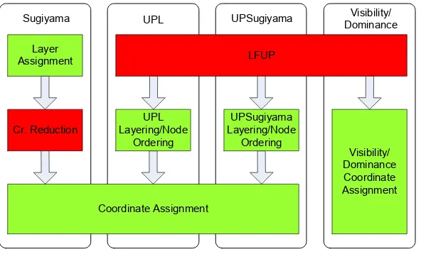
Overview of the Frameworks. We give here an overview of the drawing algo-rithms we encountered in our experiments (cf. Fig. 2). They are: the classical Sugiyama framework (Sugiyama), our new upward planarization layout (UPL), the straight-forward approach (UPSugiyama), and the dominance and visibility drawing approaches (Dominance and Visibility). An example drawing of each approach is given in Fig. 3.
When considering the layer assignment as a sub-step of coordinate assignment, the drawing frameworks based on upward planarization can be properly divided into two main phases: The crossing minimization and the coordinate assignment phase. The coordinate assignment phase ofUPL and UPSugiyama can further be divided into two sub-steps: the layering/node ordering step and final coordinate assignment.
Upward Planarization. We briefly sketch the upward planarization approach pro-posed in [8]. It can be divided into two phases: the feasible subgraph computation and the reinsertion phase. In the first phase the input DAGGis transformed into a single-source digraphG′ by adding an artificial super source ˆs and connecting it to
the sources of G. Then we compute a spanning tree T of G′ and iteratively try to
insert the remaining arcs intoT. Thereby, we perform a subgraph feasibility test after each inserted arce: we not only test upward planarity but also if all remaining edges can potentially still be inserted (with crossings) in an upward fashion. If the resulting digraph is not feasible in this sense, we adde to a set of deleted arcsB instead. By applying these operations, we obtain an embedded feasible upward planar subgraph
U.
In the second phase, the arcs inBare reinserted intoUone after another such that few crossings arise. Thereby, the crossings caused by the reinsertion are replaced by crossing dummies. As a result, we obtain an upward planar representation ofG′. This
Layer Assignment
Cr. Reduction
Coordinate Assignment
LFUP
Visibility/ Dominance Coordinate Assignment UPL
Layering/Node Ordering
UPSugiyama Layering/Node
Ordering
Sugiyama UPL UPSugiyama Visibility/ Dominance
Figure 2: Overview of the frameworks: the classical drawing framework by Sugiyama et al. (Sugiyama); our new upward planarization layout approach (UPL); the straight-forward application of the Sugiyama framework on the upward planar representation
(UPSugiyama); the dominance and visibility approach (Dominance and Visibility).
For the latter three drawing algorithms we use the layer free upward crossing min-imization approach (LFUP) by Chimani et al. [8] for obtaining an upward planar representation.
The runtime of the first phase is O(|A|2) and the runtime for the second phase O(|A|5). Therefore, an upward planarized representation for any connected DAG
G= (V, A) can be computed in timeO(|A|5).
In the following, an upward planar representation is always an augmented embed-ded graph R. Letv ande be a node and an arc in G, respectively. We denote the corresponding node and arc inR byvRandeR, respectively.
Organization of the Paper. In Sect. 2, we show how to perform layer, node order, and coordinate assignment using an upward planar representation, as well as some further beautifications. In Sect. 3, we experimentally evaluate our algorithm and compare it with existing approaches and in Sect. 4 we give a conclusion on the new drawing method. Sect. 5 shows some example drawings, comparing the results obtained by our approach with drawings produced by applying the classical Sugiyama framework.
2
Upward Planarization Layout Algorithm
LetRbe an upward planar representation of a DAGG. LetD∗be an upward drawing
induced byR such that all crossing dummy nodes are replaced by crossings and all auxiliary arcs and nodes are omitted. A drawingD is a realization of R if for each nodev ofG, the arc order ofvinduced byDcoincides with the arc order induced by
D∗and the crossings arising inDare the ones modeled byR.
1 2
7
5
0
9 4 6
3
8
3
2
1
0 4
5 6
7 8
9
4
8
7 6
2
0
5
9 3
1
6
2 5
1
7 3
4
8 9
0 4
5 6
7
8 9
3
2
1
0 (a)
(b)
(c)
(d)
(e)
10
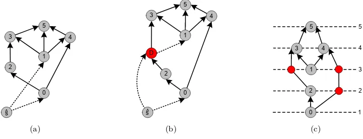
Figure 4: Illustration of the upward planarization approach by Chimani et al. [8]: (a) input DAG G augmented to G′ via the artificial super source ˆs; (b) embedded
feasible subgraphU of G′ obtained by deleting the arcs (10,13),(2,14),(4,3),(6,5);
(c) upward planar representationR of Gafter reinserting the deleted arcs (dashed line). R contains five crossing dummies. By adding sink-arcs (drawn with hollow arrow heads) and the super sink ˆt,Rbecomes a single-source, single-sink digraph.
Proposition 1 Given an upward planar representationR of a DAGG, there exists
a layering of the nodes ofG, a node order per layer, and a node placement including
bend points, such that the thereby induced drawing ofGrealizesR.
We observe that a realizing drawing ofGhence follows Sugiyama’s framework, but the individual steps do not simply optimize their respective objectives but follow the overall goal of simulating R. Our algorithm hence divides naturally into the three steps known from Sugiyama’s framework, whereby the first two steps are closely related.
As sketched in Sect. 1 (and investigated in the experimental comparison; see Sect. 3.1), it is easy to find some solution that realizes R. Yet, even if G is only of moderate size, Rcan become much larger due to the number of inserted dummy nodes. This causes weak runtime performance, many layers, and overall unsatisfac-tory drawings. Hence our algorithm aims at minimizing the required layers, thereby also reducing the necessary dummy nodes resulting from splitting long arcs.
2.1
Layer Assignment and Node Ordering
Layer Assignment. LetHbe a copy ofGthat we will use to obtain a valid layering forG; cf. Fig. 5. For any two nodes u, v ∈V(G), we add an auxiliary arc (u, v) to
H, i.e.,H =H+ (u, v) if: (a) there exists no directed path fromutov in Gand in
H, but (b) there exists a directed path fromuR to vR in R. Part (a) prohibits the
10 11 14
13
8
15
12
9 0
1 7
3
2 5
6
4
(a) The auxiliary digraphH with respect to Rfrom
Fig. 4. Arcs inH but not inGare drawn as dotted
lines.
8
15
7
10 11 12
9 0 1 2
4
14 3
6
5
13
1 2 3 4 5 6 7 8 9 10
(b) Layering ofH. Long-arc
dum-mies are drawn as smaller circles.
Figure 5: Layer Assignment and Node Ordering
ofRis mapped toH. SinceGandRare DAGs,H is also acyclic and we can use any existing layering algorithm on H. LetL =hL1, L2, ..., Lℓibe a layering for H, and
therefore also forG; i.e., ˙S1≤i≤ℓLi =V(G). We can extend this layering naturally,
by splitting any arc that spans more than one layer into a chain of arc segments by introducing dummy nodes (long-arc dummies).
Node Ordering. Considering the layering L, we now have to arrange the nodes on each layer according to the order induced byR. For this purpose, we consider the order of the arcs around each node, as given byR. In particular, we can recognize
theleft incoming arc for any nodev, which is the embedding-wise left-most arc with
targetv. Note that this arc is defined for each node except for the super source. Now consider any two distinct nodes uandv on the same layer. We can decide their correct order using the following strategy: we construct a left path pu from ˆs
touR from back to front, i.e., starting atuR we select its left incoming arceas the
end of pu and proceed from the source node of e, choosing its left incoming arc as
the second to last arc inpu, and so on. The construction ofpu ends when we reach
the super source, which will always happen asR is a single-sink DAG. Analogously, we construct the left pathpv from ˆstovR.
The pathspuandpvmay share a common subpath starting at ˆs; letcRbe the last
common node ofpu andpv, and leteu andevbe the first different arcs, respectively.
We determine the ordering ofuand v directly by the order ofeu and ev at cR. For
example in Fig. 5, ifu andv are the nodes ‘4’ and ‘12’ respectively (layer 5), then node ‘ˆs’ is the last common node of their corresponding left paths inR(see Fig. 4(c)), and hencev is left ofu.
not already “solved” by other arcs through transitivity. We obtain a final layering realizingR.
The height of a layeringL is the number of layers of L. Our layering algorithm above has the following property:
Lemma 1 LetR be an upward planar representation of a single-source DAGGand
La layering realizing Rsuch that Lis obtained by applying a longest path algorithm
onH. Lethbe the height ofL. Then for any layeringL′with heighth′,h≤h′ holds.
Proof:
Letpbe a directed path from uR tovRin Rsuch that there is no corresponding
directed path fromutov inGandH (condition (a)). For convenience we identifyp
with a sequence of arcse1, . . . , ek. Notice that an arc ei of pcannot be adjacent to
the super sink ˆtofR, since ˆtis not a node ofG. Also,eiis not associated with an arc
added for connecting the super source with the sources ofG, sinceGis a single-source digraph.
We prove by induction over k that adding an auxiliary arc a = (u, v) to H is necessary in order to ensure the hierarchy order between nodeuandv. In particular,
acannot be omitted if the layering Lshall realize R.
Induction basis (k= 1): pcontains only one arc e1 = (uR, vR). Since uR andvR
are not crossing dummies,e1is not an arc segment of any arc. (An arc segment arises
by splitting an arc during the upward planarization.) Also,e1 does not correspond
to a “real” arc of G due to condition (a); thus e1 is a sink-arc. u is a sink (
sink-switch) andv is the topmost node (top-sink-switch) of an inner facef of an upward
planar drawing ofR. Obviously, v must be drawn higher thanu in a realization of
R. Therefore adding arc ato H ensures the hierarchy order between uandv. Induction step: We assume that the hierarchy order of the nodes ofp′ =e
1, . . . , ej
withj < kis mapped toH by adding some auxiliary arcs to it.
Letp=e1, . . . , ek withek = (xR, vR). There are three possible cases:
(i) ek is a sink-arc: The fact that xis layered higher than uis already mapped
to H (induction assumption). Sinceek is a sink-arc,v must be layered higher
thanx(see induction basis), and therefore higher than u. Adding arc ato H
ensures the hierarchy order.
(ii) There is a “real” arc (x, v) in G corresponding to ek: By the induction
as-sumption the hierarchy order betweenuandxis mapped toH by adding some auxiliary arcs. Hence there is a path from utoxin H and, sinceH is a copy of G, there is also a path fromu tov. Due to condition (a) no auxiliary arcs are added toH.
(iii) ek is an arc segment: xR is a crossing dummy and the target node of arcek−1.
We have two sub-cases:
Caseek−1 andek are arc segments of a common arcb= (w, v), b∈G: By the
induction assumption, the hierarchy order between nodeuandwis mapped to
H. Sincewmust be layered higher than uand since the arcb= (w, v) exists,
v must be layered higher thanwand therefore higher thanu. Adding arcato
0 1 3
5
2
4
s ^
(a)
0 1 3
5
2
4
s ^ D
(b)
2 5
4 3
1
1 2 3 4 5
0
(c)
Figure 6: An example of a layering with unnecessary layers: (a) input DAGGwhich is augmented to an sT-graph; (b) an upward planar representation R of G; (c) a layering ofGrealizingR obtained by our layering and node ordering approach. The number of layers can be reduced by one if we assign node ‘1’ to layer 2 (as the right neighbor of node ‘2’), node ‘3’ and ‘4’ to layer 3, and node ‘5’ to layer 4.
Case ek−1 andek are not arc segments of a common arc: Letek−1 be an arc
segment of arcd= (w,·) andekbe an arc segment of arcb= (·, v). The crossing
dummyxRmodels the crossingξbetween arcband arcd. Thereforeξmust be
drawn higher thanwin an upward drawingDandvmust be drawn higher than
ξ; otherwise the line segment fromξ tov in Dwould not point monotonically increasing in the vertical direction. Thusv must be layered higher thanu. We have to add the arcato H to reflect this fact.
The induction proof reveals that no additional auxiliary arcs ofH can be omitted; otherwise the hierarchy order of the nodes may not be mapped toH correctly. Hence a layeringL with respect toR obtained by applying a longest path algorithm to H
contains no unnecessary layers. After computing the node order and rearranging the nodes ofL,Lis a realization ofR.
Unfortunately, our layer assignment approach can compute a layering with un-necessary layers for DAGs with multiple sources. Fig. 6 gives an example for such a case. The path from node ‘2’ to node ‘1’ arises in the representation due to the arc (ˆs,1). Therefore, node ‘1’ is layered higher than actually necessary.
2.1.1 Long-Arc Dummy Reduction
Adominated subgraphofGw.r.t. a nodesis the subgraph induced by the nodesvfor
Figure 7: A drawing of graphgrafo2379.35 (Rome graphs): (left) without postpro-cessing, (right) after applying source repositioning (white node) and long-arc dummy reduction (black node).
We tackle this problem using an approach similar to thepromotion node method
by Nikolov and Tarassov [17] by re-layering parts of the dominated subgraphs after the removal of ˆs, without modifying the hierarchical order induced byR. Layers that become empty by these operations can be removed afterwards:
For EachsourcesinG(in decreasing order of their layer indexj):
(a) Mark the subgraph dominated bys. LetMibe the marked nodes on layer
Li (1≤i≤ℓ).
(b) Fori=j+ 1 Toℓ:
If Mi are all long-arc dummiesThen
(i) Remove the nodesMi and lift the marked subgraph on the layers
below Li by one layer.
(ii) If the new layering causes more edge crossingsOrmore long-arc dummies Then Undo step (i) and Break (continue with next source)
2.1.2 Repositioning the Sources
21 18
16 17
10
11 0 14
12 23
3 2 7
6
1
9 8
13 22 20
15 4
5 19 19
23 4
17 10
12
11 8
14
1 6
16
20 22 13
7
9
21
3 15
2 0 18 5
Figure 8: A drawing of graphgrafo159.24 (Rome graphs) with random node sizes: without (left) and with (right) our bending arcs method and individual layer distance assignment.
2.2
Coordinate Assignment
After the previous steps we get a correct layering and node ordering realizing R. Conceptually, we can useanycoordinate assignment strategy (e.g., [6, 13]) known for Sugiyama’s layout algorithm; it will always preserve the given number of crossings. All these methods assign horizontal coordinates to the nodes while preserving the given node ordering on each layer. The aim is to generate drawings such that the subdivided long arcs are drawn as vertical straight lines for their most part.
Yet, when considering the hard-to-measure “beauty” or “readability” of the re-sulting drawings, we realize that we can improve on traditional coordinate assignment strategies as they usually do not accommodate the following two drawing problems:
• node-arc crossings: A line segment connecting nodes or bend points between
layer Li and Li+1 may cross through some nodes of these two layers. This
can easily happen when node sizes are relatively large compared to the layer distance.
• long-line segments: The general direction of upward drawings should naturally
be along the vertical direction. Yet, there can be arc segments between some layersLi and Li+1 which are very long since they span a large horizontal
dis-tance. Such arcs can make Sugiyama-style drawings hard to read.
Fig. 8 shows the benefit of the two strategies described below. Note that these strategies are not only applicable to our layout algorithm, but to any Sugiyama-style layout.
2.2.1 Vertical Coordinates
Usually, the vertical coordinates for the nodes on layerLi are simply given byδ·i,
where δ is the minimal layer distance. Yet, often we may prefer larger distances between layers in order to improve readability: larger distances counter both above problems, but in our context we are in particular interested in long-line segments—we will discuss how to tackle node-arc crossings in Sect. 2.2.2.
Layer i+1
u w
a c v Layer i
Height(a)/2
d e
Layer i v
u
d Height(a)/2
Figure 9: Avoiding node–line overlapping by introducing new bend points into an arc
e(top); horizontal coordinates of bend points must all be distinct, even if all involved arcs require a bend (bottom).
Let σi be the number of arcs between Li and Li+1 whose lengths are at least
3δ. We set the vertical distance between these two layers to (1 + min{σi/4,2})δ
(empirically evaluated).
2.2.2 Bending Arcs
While enlarging the layer distance also helps to prevent node–line crossings, the required increase in height is usually not worth it—from the readability perspective. We therefore propose a strategy that allows trading additional bend points for layer distance. The strategy can be parameterized to find one’s favorite trade-off between these two measures, namely, increase the layer distances to reduce the number of bend points or keep the layer distances small, instead introduce new bend points to avoid node–line crossings.
Let X(v) and Y(v) denote the horizontal and vertical coordinates of a node v, respectively. An arc (or line segment) e = (v, w) is pointing upward from left to
right (right to left) ifX(v)< X(w) (X(v)> X(w), resp.). Since purely vertical line
segments cannot cross through nodes, we distinguish four cases: eis pointing upward from right to left (or left to right) and v (or w) is a node on layer i. In all these cases,ehas to bend if it overlaps some nodes ofLi. However, bendingemight cause
additional crossings. To avoid this, we also have to bend the line segments that cross the just bended line. W.l.o.g., we only discuss the caseX(v)> X(w) with v ∈Li.
The other cases can be solved analogously.
Let width(v) and height(v) denote the width and height of the bounding box of a node v. Let a be the node on layer Li with the highest bounding box, and let α:= height(a)/2. Ifvis a bend point and not shifted downwards before, then we do not need to introduce an additional bend. Instead we movevupwards byα. Ifv was already shifted downwards before due to one of our other cases, then we bende by introducing a new bend point b and setX(b) :=X(v) and Y(b) :=Y(v) + 2α. We observe: By settingY(v) to αor in the latter case, setting the new bend pointb to
Y(v) + 2α, we ensure thatecannot overlap any nodes on layerLi.
e. Thereby we have to consider that other arcs might also get rerouted and so we must accommodate enough space for them as well, such that no two bend points may coincide. In particular, it might be that the arcs leavingv’s left neighbor to the right might also require additional bend points (cf. Fig. 9). Let u be the left neighbor of v on Li and d := X(v)−X(u)−width(v)/2−width(u)/2 their inner distance.
Letr be the number of line segments adjacent tov and pointing from right to left; among these, assume that e is the j-th segment when counting from left to right. Letq be the number of line segments adjacent touand pointing from left to right. Then, ∆ := d
q+r+1 gives the distances between the potential bend points, and the
coordinates of the new bend pointb are:
X(b) := X(u) +width(u)
2 + ∆·(j+ min{q, j−1})
Y(b) := Y(v) +α
In the worse case we have to introduce a new bend point for each line segment in order to prevent overlapping of the bend points and to prevent newly arising crossings (cf. Fig. 9 (bottom)). Therefore the number of newly introduced bend points for a layer Li is bounded by the number of line segments connecting the nodes or bend
points ofLi andLi+1.
3
Experiments
We investigate the quality of our new algorithm in comparison with known algo-rithms. We first compare different approaches to draw a computed upward planar representation, i.e., if the crossing number is the most important factor in our draw-ing. Afterwards, we also compare our approach to Sugiyama’s traditional framework. All algorithms are implemented in the free and open-source (GPL) Open Graph
Drawing Framework (OGDF) [18]. The experiments were conducted on an Intel
Pentium 4 3.4Ghz PC with 2GB of RAM. All data points of the diagrams represent average values for the corresponding node or density group respectively. We use the following benchmark sets:
Rome Graphs: The Rome graphs [10] are a widely used benchmark set in graph drawing, which was obtained from a basic set of 112 real-world graphs. It contains 11528 instances with 10–100 nodes and 9–158 edges. Although the graphs are originally undirected, they have been used as directed graphs by artificially directing the edges according to the node order given in the input files [12, 8].
North DAGs: The North DAGs1 have been introduced in an experimental
com-parison of algorithms for drawing DAGs [9]. The set consists of 1277 DAGs collected by Stephen North.
Since the North DAGs are a collection of heterogeneous digraphs, that is, the density of the digraphs with same number of nodes may vary from very dense to very sparse, we decided to group the DAGs into 9 sets, where the first set contains digraphs with 10 to 20 nodes and thei-th set contains digraphs with 10i+ 1 to 10(i+ 1) nodes fori= 2, . . . ,9.
Random DAGs: The real-world origin of the above benchmarks results in sets where, e.g., the relative graph densities (i.e., the ratio |A|/|V| for a digraph
G = (V, A)) are not uniformly distributed over the different graph sizes; in particular larger graphs tend to have lower densities. For a deeper investiga-tion of our algorithm regarding graphs with high densities, we use a set of 200 random DAGs previously generated by us [7]. Each DAG has 100 nodes and each potential arc occurs with uniform probability p. The DAGs are grouped in 10 subsets such that each subset is generated with a certainpcorresponding to the expected density̺=|A|/|V| ∈ {1.5,2,2.5, . . . ,6}.
Although most real-world graphs have a density below 2–3, evaluating the draw-ing algorithms for these random DAGs can reveal some theoretical insight into the behavior of these algorithms.
3.1
Planarization Layouts
As outlined in the introduction, there are various other possibilities to draw an upward planar representationRof a digraph. Therefore, we useRalso as input for alternative drawing algorithms. After computing the drawing, we can replace the dummy nodes by usual arc crossings and remove the sink-arcs and the super source/sink. By this approach we guarantee that the resulting drawing realizes the specified representation. We compare the new drawing algorithmUPLto the dominance drawing style [11]
(Dominance), the visibility representation drawing style [19] (Visibility), and a
straight-forward application of Sugiyama’s framework (UPSugiyama). For the latter, we use an optimal ranking [13] for layering, extract the node orders directly from the upward planar representation, and apply the coordinate assignment algorithm by Buchheim et al. [6].
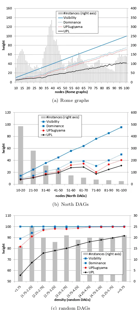
Fig. 10 and Fig. 11 show the average heights and widths of the resulting drawings for the Rome graphs, the North DAGs, and the random graphs, respectively. The average aspect ratios (i.e., the ratio width/height) of the drawings are given in Fig. 12. For a fair comparison between the different approaches, we want to disregard any differences which are only due to spacing parameters. Therefore, we use the following conventions: The height of a drawing is simply the number of required layers (in case ofUPL and UPSugiyama) or the number of vertical grid coordinates (in case
ofDominance andVisibility), respectively. Thewidth of a drawing is the maximum
number ofelements per layer or horizontal grid line, respectively, where the elements on a layer or grid lineℓare the nodes on ℓas well as the edge lines crossingℓ.
For a fair runtime comparison, we use the same coordinate assignment algo-rithm [6] forUPLandUPSugiyama. This choice is due to the fact that the alternative LP-based approach [13] requires too much time for UPSugiyama, because it has to consider very large digraphs due to the crossing and long-arc dummies. Note that the height and width measures defined above are invariant under the choice of the coordinate assignment algorithm. The average runtimes (in seconds) are shown in Fig. 13. We omit showing runtimes for the linear-time algorithms Dominance and
Visibility, since they are usually below any measurable threshold. Instead, we give
their average and maximum runtime values in Table 1.
0
nodes (Rome graphs)
#instances (right axis) Visibility
Dominance UPSugiyama UPL
(a) Rome graphs
0
10-20 21-30 31-40 41-50 51-60 61-70 71-80 81-90 91-100
h
e
ig
h
t
nodes (North DAGs)
#instances (right axis) Visibility
Dominance UPSugiyama UPL
(b) North DAGs
0
density (random DAGs)
#instances (right axis) Visibility
Dominance UPSugiyama UPL
(c) random DAGs
0 50 100 150 200 250 300 350
0 10 20 30 40 50 60 70
10 15 20 25 30 35 40 45 50 55 60 65 70 75 80 85 90 95 100
w
id
th
nodes (Rome graphs)
#instances (right axis) Dominance UPSugiyama Visibility UPL
(a) Rome graphs
0 100 200 300 400 500 600
0 10 20 30 40 50 60
10-20 21-30 31-40 41-50 51-60 61-70 71-80 81-90 91-100
w
id
th
nodes (North DAGs)
#instances (right axis) UPSugiyama Dominance Visibility UPL
(b) North DAGs
0 5 10 15 20 25 30
0 50 100 150 200 250 300
w
id
th
density (random DAGs)
#instances (right axis) UPSugiyama Visibility Dominance UPL
(c) random DAGs
0
nodes (Rome graphs)
#instances (right axis) UPL
UPSugiyama Dominance Visibility
(a) Rome graphs
0
10-20 21-30 31-40 41-50 51-60 61-70 71-80 81-90 91-100
a
nodes (North DAGs)
#instances (right axis) UPSugiya UPL Dominance Visibility
(b) North DAGs
0
nodes (random DAGs)
#instances (right axis) UPL
UPSugiyama Dominance Visibility
(c) random DAGs
0
nodes (Rome graphs)
#instances (right axis) UPSugiyama UPL
(a) Rome graphs
0
10-20 21-30 31-40 41-50 51-60 61-70 71-80 81-90 91-100
ti
nodes (North DAGs)
#instances (right axis) UPSugiyama UPL
(b) North DAGs
0
density (random DAGs)
#instances (right axis) UPSugiyama UPL
(c) random DAGs
Rome graphs North DAGs random DAGs
Algorithm avg max avg max avg max
Visibility 0.00067 0.016 0.00032 0.016 0.138 0.438 Dominance 0.00055 0.060 0.00039 0.032 0.122 0.390
Table 1: Average and maximal runtime ofVisibility andDominance in seconds.
number of nodes the length of the longest path also increases. The diagram for the North DAGs (Fig. 10(b)) contains an unusual break at node group 71–80. The reason is that this group is the group with the shortest average longest path and the lowest average density. Furthermore, we observe that the heights of the drawings increase when the graphs becoming denser. Also the gap betweenUPLand the other planarization algorithms decreases; see Fig. 10(c). As the density increases, the height converges to the maximal possible height (see Fig. 10 (c)). Concerning drawing width
UPLis clearly the winner on the Rome and North graphs benchmark sets, while all algorithms perform nearly the same on the random DAGs. As expected, the width increases when the instances becoming denser or when the number of nodes increases. This is due to the fact that digraphs with high numbers of nodes “need” more layers, and thus there are more arcs spanning more than one layer. Hence, the number of long arc dummies on a layer increases. If a digraph has a high density then more long arc dummies occur and the width also increases. For the same reason the aspect ratio of the random DAGs increase when the instances becoming denser. Regarding the runtimeUPLis the clear winner compared toUPSugiyama (cf. Fig. 13).
3.2
Comparison with Traditional Sugiyama
Finally, we can investigate how much the requirement of having a drawing with few crossings costs in terms of other quality measures. Therefore we compareUPLto a traditional Sugiyama approach that is not bound to a specific upward planar repre-sentation. For the latter we use the experimentally most competitive algorithms for the individual steps: We use the optimal LP-based approach for layering [13], the barycenter heuristic for the crossing reduction step (with best of 5 randomized runs), and assign the coordinates via the exact LP-based approach [13]. For a fair compari-son,UPLalso applies the LP-based coordinate assignment algorithm. This time, the runtime ofUPLincludes also the computation of the upward planar representation, because this step is not necessary forSugiyama. We remark that the implementation of the planarization was vastly improved compared to previous results [8].
Clearly, the number of crossings in the pure Sugiyama approach is much higher (Fig. 14), which complies with the findings in [8]. As shown in Fig. 15,UPL’s drawings are of course higher than Sugiyama’s by construction. Like for the planarization layouts, the width and height of Sugiyama drawings increases when the number of nodes or the density of the graphs increases. WhileUPLproduces often drawings with smaller widths for the Rome and North graphs (see Fig. 15 (a) and (b)), Sugiyama
achieved better results for the random DAGs. This is due to the lower height of
Sugiyama drawings. The Sugiyama approach requires fewer long arc dummies than
0
nodes (Rome graphs)
#instances (right axis) Sugiyama UPL
(a) Rome graphs
0
10-20 21-30 31-40 41-50 51-60 61-70 71-80 81-90 91-100
cr
nodes (North DAGs)
#instances (right axis) Sugiyama UPL
(b) North DAGs
0
density (random DAGs)
#instance (right axis) Sugiyama Upward Planarization
(c) random DAGs
0
nodes (Rome graphs)
#instances (right axis) Width - Sugiyama Width - UPL Height - UPL Height - Sugiyama
(a) Rome graphs
0
10-20 21-30 31-40 41-50 51-60 61-70 71-80 81-90 91-100
h
nodes (North DAGs)
#instances (right axis) Width - UPL Width - Sugiyama Height - UPL Height - Sugiyama
(b) North DAGs
0
density (random DAGs)
#instances (right axis) Width - UPL Width - Sugiyama Height - UPL Height - Sugiyama
(c) random DAGs
0
nodes (Rome graphs)
#instances (right axis) Sugiyama UPL
(a) Rome graphs
0
10-20 21-30 31-40 41-50 51-60 61-70 71-80 81-90 91-100
a
nodes (North DAGs)
#instances (right axis) Sugiyama UPL
(b) North DAGs
0
density (random DAGs)
#instances (right axis) Sugiyama UPL
(c) random DAGs
0
nodes (Rome graphs)
#instances (right axis) Up. Planarization+UPL Up. Planarization Sugiyama
(a) Rome graphs
0
10-20 21-30 31-40 41-50 51-60 61-70 71-80 81-90 91-100
ti
nodes (North DAGs)
#instances (right axis) Up. Planarization+UPL Up. Planarization Sugiyama
(b) North DAGs
0
density (random DAGs)
#instances Up. Planarization+UPL Upward Planarization Sugiyama
(c) random DAGs
with respect to this measure if a small number of crossings is an important issue.
UPLhas certain advantages over Sugiyama’s approach: A strong packing into few layers as produced by the Sugiyama approach will usually require a wider drawing than our planarization approach. Furthermore, such few layers can in fact be coun-terproductive regarding readability of the drawings; see, e.g., Fig. 1. Overall, we can observe thatUPL obtains a more balanced aspect ratio than Sugiyama’s approach; see Fig. 16.
In terms of running time (Fig. 17), we see that while Sugiyama’s approach is generally faster,UPLis not too slow either, requiring below 1.5 seconds for the large instances of the Rome and North graphs. However, as the density of the graphs increases the gap betweenSugiyamaand UPLincreases rapidly.
4
Conclusion
Traditional methods for drawing DAGs consider the number of crossings only as a second order priority. If it is of highest priority, one has to use algorithms based on upward planar representations. Our algorithm constitutes the first such algorithm that takes the special crossing nodes into account. As our experiments show, it generates drawings that are preferable over alternative methods for drawing upward planar representations. Furthermore, the new drawing algorithm is also compara-ble to Sugiyama’s approach with respect to other quality measures, while offering a significantly smaller number of crossings.
We conclude with two interesting open problems:
1. Regarding Lemma 1, can we archive a similar result for general (instead of only single-source) DAGs?
2. As shown by our experiments, there is a gap between Sugiyama’s and our UPL approach regarding the height of the drawings. Clearly, this gap cannot be eliminated completely, but how can we reduce this gap? This problem includes the problem of finding a suitable upward planar representation Rof the input DAGGfor a compact realization.
5
Drawings
In this section we give some example drawings produced by our new algorithmUPL
6
(a) UPL drawing of instance
g.38.21 (North DAGs) with one
crossing.
(b) Sugiyama drawing of instance
g.38.21 (North DAGs) with 27
crossings.
Figure 18: Comparison of drawings where all nodes have the same size.
49
(a) UPL drawing of instance grafo3579.53
(Rome graphs) with 9 crossings.
15
(b) Sugiyama drawing of instance
grafo3579.53 (Rome graphs) with 76
crossings.
18
(a) UPL drawing of instanceg.60.0 (North DAGs) with 82 crossings.
31
(b) Sugiyama drawing of instance g.60.0
(North DAGs) with 250 crossings.
3
(c) UPL drawing of instance
grafo8087.84 (Rome graphs) with
41 crossings.
(d) Sugiyama drawing of instance
grafo8087.84 (Rome graphs) with
134 crossings.
References
[1] C. Batini, M. Talamo, and R. Tamassia. Computer aided layout of entity rela-tionship diagrams. J. Syst. Software, 4:163–173, 1984.
[2] G. D. Battista, E. Pietrosanti, R. Tamassia, and I. Tollis. Automatic layout of PERT diagrams with X-PERT. InProc. IEEE Workshop on Visual Languages, pages 171–176, 1989.
[3] P. Bertolazzi, G. Di Battista, C. Mannino, and R. Tamassia. Optimal upward planarity testing of single-source digraphs. SIAM J. Comput., 27(1):132–169, 1998.
[4] U. Brandes and B. K¨opf. Fast and simple horizontal coordinate assignment. In
Proc. Graph Drawing ’01, pages 31–44, London, UK, 2002. Springer-Verlag.
[5] J. Branke, S. Leppert, M. Middendorf, and P. Eades. Width-restricted layering of acyclic digraphs with consideration of dummy nodes. Inf. Process. Lett., 81(2):59–63, 2002.
[6] C. Buchheim, M. J¨unger, and S. Leipert. A fast layout algorithm for k-level graphs. In Proc. Graph Drawing ’00, volume 1984 of LNCS, pages 229–240. Springer, 1999.
[7] M. Chimani, C. Gutwenger, P. Mutzel, and H.-M. Wong. Layer-free upward crossing minimization. ACM J. Exp. Algorithmics. To appear.
[8] M. Chimani, C. Gutwenger, P. Mutzel, and H.-M. Wong. Layer-free upward crossing minimization. In WEA 2008: Workshop on Experimental Algorithms, volume 5038 of LNCS, pages 55–68. Springer, 2008.
[9] G. Di Battista, A. Garg, G. Liotta, A. Parise, R. Tamassia, E. Tassinari, F. Vargiu, and L. Vismara. Drawing directed acyclic graphs: An experimen-tal study. Int. J. Comput. Geom. Appl., 10(6):623–648, 2000.
[10] G. Di Battista, A. Garg, G. Liotta, R. Tamassia, E. Tassinari, and F. Vargiu. An experimental comparison of four graph drawing algorithms. Comput. Geom.
Theory Appl., 7(5-6):303–325, 1997.
[11] G. Di Battista, R. Tamassia, and I. G. Tollis. Area requirement and symmetry display of planar upward drawings.Discrete Comput. Geom., 7(4):381–401, 1992.
[12] M. Eiglsperger, M. Kaufmann, and F. Eppinger. An approach for mixed upward planarization. J. Graph Algorithms Appl., 7(2):203–220, 2003.
[13] E. Gansner, E. Koutsofios, S. North, and K.-P. Vo. A technique for drawing directed graphs. Software Pract. Exper., 19(3):214–229, 1993.
[15] P. Healy and N. S. Nikolov. A branch-and-cut approach to the directed acyclic graph layering problem. In Proc. Graph Drawing ’02, pages 98–109, London, UK, 2002. Springer-Verlag.
[16] P. Healy and N. S. Nikolov. How to layer a directed acyclic graph. In Proc.
Graph Drawing ’01, pages 16–30, London, UK, 2002. Springer-Verlag.
[17] N. S. Nikolov and A. Tarassov. Graph layering by promotion of nodes. Discrete
Applied Mathematics, 154(5):848–860, 2006.
[18] OGDF – The Open Graph Drawing Framework. Technische Universit¨at Dort-mund, Chair of Algorithm Engineering; see http://www.ogdf.net.
[19] P. Rosenstiehl and R. E. Tarjan. Rectilinear planar layouts and bipolar orienta-tions of planar graphs. Discrete Comput. Geom., 1(1):343–353, 1986.

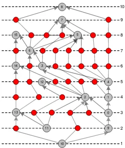
![Figure 3: Layout of instance g.10.19 (North DAGs): (a) Dominance; (b) Visibility;(c) Sugiyama; (d) UPSugiyama; (e) UPL; the drawings (a), (b), (d) and (e) are basedon a common upward planar representation produced by [8].](https://thumb-ap.123doks.com/thumbv2/123dok/930869.904212/6.612.120.485.122.622/instance-dominance-visibility-sugiyama-upsugiyama-drawings-representation-produced.webp)
![Figure 4: Illustration of the upward planarization approach by Chimani et al. [8]:(a) input DAGarrow heads) and the super sink line).(c) upward planar representationfeasible subgraph G augmented to G′ via the artificial super source ˆs; (b) embedded U of G′](https://thumb-ap.123doks.com/thumbv2/123dok/930869.904212/7.612.128.486.116.297/illustration-planarization-approach-dagarrow-representationfeasible-augmented-articial-embedded.webp)